Time Series Analysis Part I

A time series is a sequence of numerical data in which each item is associated with a particular instant in time. Many sets of data appear as time series: a monthly sequence of the quantity of goods shipped from a factory, a weekly series of the number of road accidents, daily rainfall amounts, hourly observations made on the yield of a chemical process, and so on. Examples of time series abound in such fields as economics, business, engineering, the natural sciences (especially geophysics and meteorology), and the social sciences.

• Univariate time series analysis- When we have a single sequence of data observed over time then it is called univariate time series analysis.
• Multivariate time series analysis – When we have several sets of data for the same sequence of time periods to observe then it is called multivariate time series analysis.

The data used in time series analysis is a random variable (Yt) where t is denoted as time and such a collection of random variables ordered in time is called random or stochastic process.

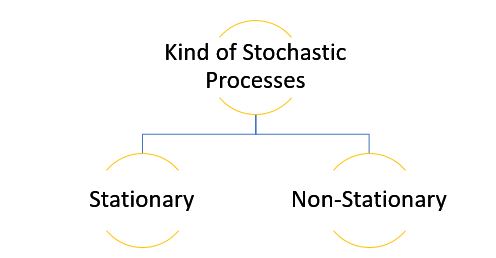
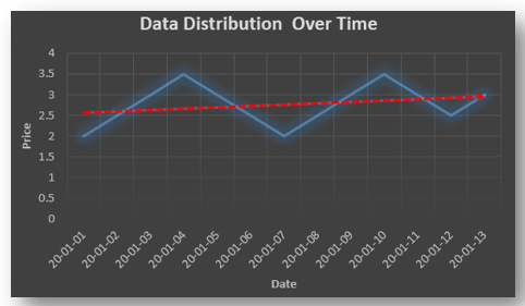
Stationary: A time series is said to be stationary when all the moments of its probability distribution i.e. mean, variance , covariance etc. are invariant over time. It becomes quite easy forecast data in this kind of situation as the hidden patterns are recognizable which make predictions easy.

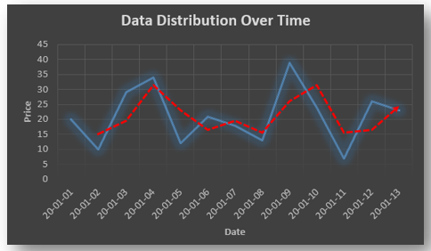
Non-stationary: A non-stationary time series will have a time varying mean or time varying variance or both, which makes it impossible to generalize the time series over other time periods.

Non stationary processes can further be explained with the help of a term called Random walk models. This term or theory usually is used in stock market which assumes that stock prices are independent of each other over time. Now there are two types of random walks:
Random walk with drift : When the observation that is to be predicted at a time ‘t’ is equal to last period’s value plus a constant or a drift (α) and the residual term (ε). It can be written as
Yt= α + Yt-1 + εt
The equation shows that Yt drifts upwards or downwards depending upon α being positive or negative and the mean and the variance also increases over time.
Random walk without drift: The random walk without a drift model observes that the values to be predicted at time ‘t’ is equal to last past period’s value plus a random shock.
Yt= Yt-1 + εt
Consider that the effect in one unit shock then the process started at some time 0 with a value of Y0
When t=1
Y1= Y0 + ε1
When t=2
Y2= Y1+ ε2= Y0 + ε1+ ε2
In general,
Yt= Y0+∑ εt
In this case as t increases the variance increases indefinitely whereas the mean value of Y is equal to its initial or starting value. Therefore the random walk model without drift is a non-stationary process.

So, with that we come to the end of the discussion on the Time Series. Hopefully it helped you understand time Series, for more information you can also watch the video tutorial attached down this blog. DexLab Analytics offers machine learning courses in delhi. To keep on learning more, follow DexLab Analytics blog.

Classroom or Online Certification Courses to get you started

To learn more about Data Analyst with Advanced excel course – Enrol NowTo learn more about Big Data Course – Enrol Now
To learn more about Machine Learning Using Python and Spark – Enrol NowTo learn more about Data Analyst with SAS Course – Enrol Now.
To learn more about Data Analyst with Apache Spark Course – Enrol Now
To learn more about Data Analyst with Market Risk Analytics and Modelling Course – Enrol Now