text analytics with python course Archives - DexLab Analytics | Big Data Hadoop SAS R Analytics Predictive Modeling & Excel VBA

Python Statistics Fundamentals: How to Describe Your Data? (Part I)

Python Statistics Fundamentals: How to Describe Your Data?

Statistics is a branch of mathematics which deals with the collection, analysis, interpretation and presentation of masses of numerical data. Statistics is a tool used to communicate our understanding of data. It helps us understand the world better, make assertions, and communicate our confidence in the statements we are making.

Two main statistical methods are used in data analysis:

  1. Descriptive statistics: This method is used to summarize data from a sample using measures such as the mean or standard deviation
  2. Inferential statistics: With this method, you can conclude data that are subject to random variation (e.g., observational errors, sampling variation).

This article is about the descriptive statistics which are used to describe and summarize the datasets. We are also going to see the available Python libraries to get those numerical quantities.

This whole topic will be covered in a series of two blogs. This first blog is about the types of measures in descriptive statistics. Furthermore, we will also see the built-in Python “Statistics” library, which has a relatively small number of the most important statistics functions.

Descriptive statistics can be defined as the measures that summarize a given data, and these measures can be broken down further into the measures of central tendency and the measures of dispersion. Measures of central tendency include mean, median, and the mode, while the measures of dispersion include standard deviation and variance.

We will cover the following topics in descriptive statistics:

  • Measures of Central Tendency
  1. Mean
  2. Median
  3. Mode
  • Measures of Dispersion
  1. Variation
  2. Standard Deviation

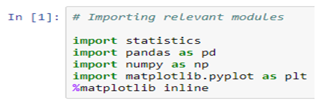
First, we need to import the Python statistics module.

Mean

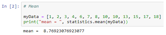
The arithmetic mean is the sum of data divided by the number of data-points. It is a measure of the central location of data in a set of values that vary in range. In Python, we usually do this by dividing the sum of given numbers with the count of the number present. Python mean function can be used to calculate the mean/average of the given list of numbers. It returns the mean of the data set passed as parameters.

mean( ): Arithmetic mean (“average”) of data.

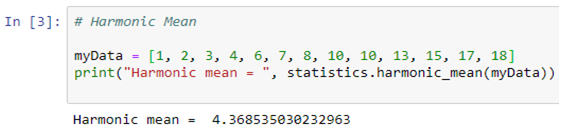
harmonic_mean( ): It is the reciprocal of the arithmetic mean of the reciprocals of the data (say for three numbers a, b and c, 1/mean = 3/(1/a + 1/b + 1/c)).
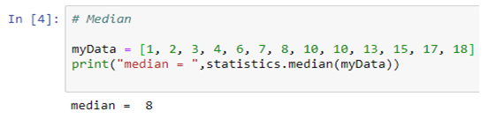
Median

median( ): Median or middle value of data is calculated as the mean of middle two. When the number of data points is odd, the middle data point is returned. The median is a robust measure of a central location and is less affected by the presence of outliers in your data compared to the mean.

median_low( ): Low median of data is calculated when the number of data points is odd. Here the middle value is usually returned. When it is even, the smaller of the two middle values is returned.

median_high( ): High median of data is calculated when the number of data points is odd. Here, the middle value is usually returned. When it is even, the larger of the two middle values is returned.
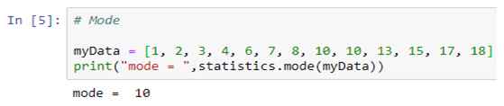
Mode

mode( ): Mode (most common value) of discrete data. The mode (when it exists) is the most typical value and is a robust measure of central location.

Measures of Dispersion

Measures of dispersion are statistics that describe how data varies, usually relative to the typical value. While measures of centre give us an idea of the typical value, measures of spread give us a sense of how much the data tends to diverge from the typical value.

These following functions (from the statistics module in python) calculate a measure of how much the population or sample tends to deviate from the typical or average values.
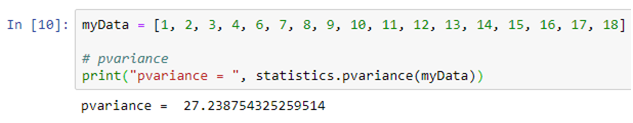
Data Science Machine Learning Certification

Population Variance

pvariance( ): Returns the population variance of data. Use this function to calculate the variance from the entire population. To estimate the variance from a sample, the variance ( ) function is usually a better choice. When called with the entire population, this gives the population variance σ². When called on a sample instead, this is the biased sample variance s², also known as variance with N degrees of freedom.

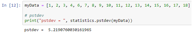
Population Standard Deviation

pstdev( ): Return the population standard deviation (the square root of the population variance)
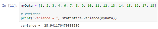
Sample Variance

variance ( ): Returns the sample variance of data, an iterable of at least two real-valued numbers. Variance, or second moment about the mean, is a measure of the variability (spread or dispersion) of data. A large variance indicates that the data is spread out; a small variance indicates it is clustered closely around the mean. If the optional second argument is given to the function, it should be the mean of data. This is the sample variance s² with Bessel’s correction, also known as variance with N-1 degrees of freedom.

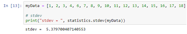
Sample Standard Deviation

stdev( ): Returns the sample standard deviation (the square root of the sample variance)

Conclusion

So, this article focuses on describing and summarizing the datasets, also helping you to calculate numerical quantities in Python. It’s possible to get descriptive statistics with pure Python code, but that’s rarely necessary. In the next series of this blog we will see the Python statistics libraries which are comprehensive, popular, and widely used especially for this purpose.


Interested in a career in Data Analyst?

To learn more about Data Analyst with Advanced excel course – Enrol Now.
To learn more about Data Analyst with R Course – Enrol Now.
To learn more about Big Data Course – Enrol Now.

To learn more about Machine Learning Using Python and Spark – Enrol Now.
To learn more about Data Analyst with SAS Course – Enrol Now.
To learn more about Data Analyst with Apache Spark Course – Enrol Now.
To learn more about Data Analyst with Market Risk Analytics and Modelling Course – Enrol Now.

Statistical Application in R & Python: Negative Binomial Distribution

Statistical Application in R & Python: Negative Binomial Distribution

Negative binomial distribution is a special case of Binomial distribution. If you haven’t checked the Exponential Distribution, then read through the Statistical Application in R & Python: EXPONENTIAL DISTRIBUTION.

It is important to know that the Negative Binomial distribution could be of two different types, i.e. – Type 1 and Type 2. In many ways, it could be seen as a generalization of the geometric distribution. The Negative Binomial Distribution essentially operates on the same principals as the binomial distribution but the objective of the former is to model for the success of an event happening in “n” number of trials. Here it is worth observing that the Geometric distribution models for the first success whereas a Negative Binomial distribution models for the Kth 

Data Science Machine Learning Certification

This is explained below.

Type 1 Binomial distribution  aims to model the trails up to and including the “kth success” in “n number of trials”. To give a simple example, imagine you are asked to predict the probability that the fourth person to hear a gossip will believe that! This kind of prediction could be made using the negative binomial type 1 distribution. 

Conversely, Type 2 Binomial distribution is used to model the number of failures before the “kth success”. To give an example, imagine you are asked about how many penalty kicks it will take before a goal is scored by a particular football player. This could be modeled using a negative binomial type 2 distribution, which might be pretty tricky or almost impossible with any other methods.

The probability distribution function is given below: 

In the next section, we will take you through its practical application in Python and R. 

Application:

Mr. Singh works in an Insurance Company where his target is to sale a minimum of five policies in a day. On a particular day, he had already sold 2 policies after numerous attempts. The probability of sales on each policy is 0.6. Now, if the policies may be considered as independent Bernoulli trials, then:

  1. What is the probability that he has exactly 4 failed attempts before his 3rd successful sales of the day?
  2. What is the probability that he was fewer than 4 failed attempts before his 3rd successful sales of the day?

So, the number of sales = 3.

The probability of failed attempts is 4.

The success of each sale is 0.6.

Calculate Negative Binomial Distribution in R:

In R, we calculate negative binomial distribution to find the probability of insurance sales. Thus, we get,

  1. The probability that he has exactly 4 failed attempts before his 3rd successful sales are 8.29%.
  2. The probability that he has fewer than 4 failed attempts before his 3rd successful sales is 82.08%.

Hence, we can see that chances are quite high that Mr. Singh will succeed in making a sale after 4 failed attempts.

Calculate Negative Binomial Distribution in Python:

In Python, we get the same results as above.

Conclusion:

Negative Binomial distribution is the discrete probability distribution that is actually used for calculating the success and failure of any observation. When applied to real-world problems, the outcomes of the successes and failures may or may not be the outcomes we ordinarily view as good and bad, respectively.

Suppose we used the negative binomial distribution to model the number of days a certain machine works before it breaks down. In this case, “success” would be the days that the machine worked properly, whereas the day when the machine breaks down would be a “failure”. Another example would be, if we used the negative binomial distribution to model the number of attempts an athlete makes on goal before scoring r goals, though, then each unsuccessful attempt would be a “success”, and scoring a goal would be “failure”.

This blog will surely aid in developing a better understanding of how negative binomial distribution works in practice. If you have any comments please leave them below. Besides, if you are interested in catching up with the cutting edge technologies, then reach the premium training institute of Data Science and Machine Learning leading the market with the top-notch Machine Learning course in India.


Interested in a career in Data Analyst?

To learn more about Data Analyst with Advanced excel course – Enrol Now.
To learn more about Data Analyst with R Course – Enrol Now.
To learn more about Big Data Course – Enrol Now.

To learn more about Machine Learning Using Python and Spark – Enrol Now.
To learn more about Data Analyst with SAS Course – Enrol Now.
To learn more about Data Analyst with Apache Spark Course – Enrol Now.
To learn more about Data Analyst with Market Risk Analytics and Modelling Course – Enrol Now.

An All-Inclusive Guide on Python and its Changing Trends

An All-Inclusive Guide on Python and its Changing Trends

Python is an extremely readable and versatile high-level programming language. Many companies such as Google, YouTube, Dropbox use the language for developing applications. It also finds its use extensively in diverse fields as in Python for data analysis, Machine Learning Using Python, Natural Language Processing, Web Development, Scientific Computing, Image processing, Robotics, Computer Vision and many more.

It supports both Object-oriented programming and Functional programming. Python is generally referred to as an interpreted language which implies that each line of code is executed one by one and if the interpreter finds an error, it stops immediately with an error message on the screen.

Another important feature of Python is its interactive prompt. A Python statement can be typed and immediately executed, which is in sharp contradiction to any other compiled language.

What are Python 2.x and Python 3.x?

There are two main versions of Python: Python 2.x and Python 3.x. If someone is new to Python, then he/she might be in confusion about which version to use. However, in the current scenario, we can easily migrate from Python 2 to Python 3, as the Python Software Foundation has finally taken the step to formally announce that Python 2 will reach the end of life (EOL) on January 1st, 2020.

Key differences between Python 2.x and Python 3.x

This article discusses the differences between these two versions of Python, making Python 3 less confusing for a new programmer.

  1. Print Function

In Python 2, print is a statement. There is no need of parenthesis.

In Python 3, print is a function. It needs parenthesis.

  1. Integer Division

In Python 2, if the division operator is performed on two integers, then the output will be an integer for example: – 7/3 = 2.

In Python 3, if the division operator is performed on two integers, then the output will be accurate. It can also be in float for example: – 7/3 = 2.33.

To get the result in an integer only a different division operator is used that is (//) it returns an integer result for example, – 7//3 = 2.

 3. Unicode Support

Both the versions of Python can handle strings (sequences of characters) differently.

Python 2 uses the ASCII encoding standard by default. ASCII is limited to representing 256 characters. This limits the flexibility of Python to encode the characters, particularly non-standard ones. Using Unicode in Python 2 requires extra syntax—for example when using print, the input text is to be wrapped in the Unicode() function to handle special characters.

In Python 3, Unicode is the default. The Unicode standard is much more versatile—it supports over 128,000 characters. There is no need for an extra syntax to define the Unicode values—they get printed automatically as utf-8 strings.

  1. Range Function

In Python 2, the range function returns a list of numbers.

In Python 2, the xrange class represents an iterable that provides the same object.

 In Python 3, original range function is removed and xrange is renamed to range:

In Python 3, it is needed to convert the range object to a list if someone desires the same result as the range function provides in Python 2.

  1. ­­­­Input() Method

Mainly what is expected from the input() method is that it reads input as string, then it can be converted into any datatype as per the requirement.

In Python 2, it has both the input() and raw_input() methods for taking input. The difference between the raw_input() and input()is that the raw_input() reads input as a string while the input() reads input as string only if it is inside quotes else reads as an integer.

In Python 3, there is no raw_input() method. The raw_input() method is replaced by input() in python 3. 

If someone still wants to use the input() method like in python 2, then it can be availed by using eval() method.

There are many other differences between Python 2 and Python 3 like: –

  1. Next() Method

In Python 2, .next() method is used and in Python 3 next() function is used to iterate the next element of an iterator.

  1. Raising Exception

To raise an exception in Python 3, the argument should be in parenthesis, while in Python 2, it is not necessary.

  1. Handling Exception

Handling exception is also changed in Python 3, “as” keyword is used in Python 3, while it is not necessary in Python 2.

So, if someone is a beginner, then it is strongly recommended to use Python 3 because it is the future of Python and also January 1, 2020, will be the last day of Python 2. It means that no improvement will be done anymore after that day, even if someone finds a security problem in it.

Data Science Machine Learning Certification

It is highly recommended to upgrade the version of the programming language to Python 3. Some ways can help the Python 2 users in porting their code from Python 2 to Python 3 and get the feel of Python 3 and figure out how it is different from Python 2. The code can be imported by using tools like “Futurize” and “Modernize”. Also, if someone wants to check the availability of Python 3 as part of his tests, then “caniusepython3.check()” can be used.

As a final note, everyone must look for upgrading their Python version to Python 3 to understand the subtleties of the new version and usher in the future. However, if you are interested in Deep learning for computer vision with Python and similar courses, then opt for the premium Python training institute in Delhi now!


.

Statistical Application in R & Python: Poisson Distribution

Statistical Application in R & Python: Poisson Distribution

Continuing with the series of blogs, the first of which was Statistical Application In R & Python: Normal Probability Distribution, here we bring you a post on how you can calculate Poisson distribution effortless using R & Python. So, stay tuned!

Poisson distribution is a counting process which is a discrete probabilistic model. It has only one parameter, (lambda or “m”) which is essentially the average rate of change. Poisson distribution is used to model “number of anything”. The probability distribution function of a Poisson distribution is given by the below expression.

If m is the mean occurrence per interval, then the probability of having x occurrence with in a given interval is:

Application:

A business firm receives on an average 6.5 telephone calls per day during the time period 11:00 – 11:15 A.M., Find the probability that on a certain day, the firm receives exactly9 calls during the same period.

The random variable x is the ‘number of telephone calls received during the period 11:00 – 11:15 A.M, since x is assumed to Poisson distribution. The parameter m is equal to the mean of the distribution; i.e.  m = 6.5 and x = 9, then the equation is:

Calculate Poisson Distribution in R:

So, while calculating Poisson distribution in R, we notice that the probability of occurring exactly 9 calls instead of average 6.5 calls in a given particular time (11:00 A.M – 11:15 A.M ) = 85.81%

Calculate Poisson Distribution in Python:

So, while we calculate Poisson distribution in Python, we notice that the probability of occurring exactly 9 calls instead of average 6.5 calls in a given particular time (11:00 A.M – 11:15 A.M) = 85.81%

Conclusion:

Companies can use the Poisson distribution to contrive effective steps to improve their operational efficiency. For instance, an analysis done with the Poisson distribution might reveal how a company can arrange staffing in order to be able to handle the peak periods efficiently, when the customer service calls keep on pouring.

In this problem we see that the business firm receives on an average 6.5 telephone calls per day during the time period 11:00A.M – 11:15A.M, then the probability of the firm receives exactly 9 calls in a same is 85.81%.

Dexlab Analytics is the best Python training institute in Delhi, bringing you the all-inclusive courses of Python for Data Analysis and R Predictive Modelling Certification, among others to start your career in Data Science and Analytics.


Interested in a career in Data Analyst?

To learn more about Data Analyst with Advanced excel course – Enrol Now.
To learn more about Data Analyst with R Course – Enrol Now.
To learn more about Big Data Course – Enrol Now.

To learn more about Machine Learning Using Python and Spark – Enrol Now.
To learn more about Data Analyst with SAS Course – Enrol Now.
To learn more about Data Analyst with Apache Spark Course – Enrol Now.
To learn more about Data Analyst with Market Risk Analytics and Modelling Course – Enrol Now.

A Nifty Guide to Initiate AIOps in 2019

A Nifty Guide to Initiate AIOps in 2019

AIOps (artificial intelligence for IT operations) is the buzz word of the 21st century.

In this digitally-charged world, AIOps platforms are the key. They fuse ML and big data functionalities to boost and partly replace primary IT operations’ programs, including event correlation and analysis, performance monitoring and IT service automation and management.

In simple terms, AIOps is the combined application of data science and machine learning to help mitigate IT operations-related challenges and find faster insights. It fixes high-severity outages in a jiffy. 

The main objective of revolutionary AIOps platforms is to ingest and analyze the aggravating volume, variety and velocity of data and deliver it in a useful manner.

Deep Learning and AI using Python

IT bigwigs are excited about the prospects of applying AI and ML to IT operations.

Gartner expects that big enterprises’ usage of AIOps and other monitoring tools and applications will rise from 5% in 2018 to 30% in 2023. The long-term impact of AIOps on IT operations is predicted to be transformative.

Fortunately, AI capabilities are making headway, and more real-time solutions are being formulated and made available each day.

Read on to know how to get started with AIOPs:

Be prepared

First and foremost, you have to familiarize yourself with all the ML and AI capabilities and vocabulary. It doesn’t matter if you are gearing up for an AIOps project or not. Capabilities and priorities change; so be ready to implement the platform anytime soon.

Select the first few test cases carefully

Small and steady wins the race. The same phrase applies to transformation initiatives. They start small, seize knowledge and iterate from there. Imbibe the same approach for AIOps success.

Enhance your proficiency

Decode the intricacies of AIOps amongst your colleagues by displaying simple techniques. Ascertain your skills and identify the loopholes, then devise a relevant plan to fill up those gaps in-between.

Feel free to experiment

Although a majority of AIOps platforms are complex and costly, there is a substantial number of open-source and relatively low-cost ML software available in the market that lets you evaluate the efficacy of AIOps and ML applications and their uses.

Look beyond IT

Don’t forget to leverage all kinds of data analytics resources available in your organization. Data management is the cornerstone of AIOps. Most of the teams are already skilled in it. Statistical analytics and business analysis are key components of contemporary business frameworks, and many techniques traverse public domains. 

2

Standardize and modernize, as and when required

Prepare your work infrastructure to implement a robust AIOps adoption by embracing secure automation architecture, immutable infrastructure patterns and infrastructure as code (IaC).

Interested in learning more about Machine Learning Using Python? Feel free to reach us at DexLab Analytics. We’re a premier learning platform specialized in offering in-demand skill training courses to the interested candidates.


The blog has been sourced from ― www.gartner.com/smarterwithgartner/how-to-get-started-with-aiops


Interested in a career in Data Analyst?

To learn more about Data Analyst with Advanced excel course – Enrol Now.
To learn more about Data Analyst with R Course – Enrol Now.
To learn more about Big Data Course – Enrol Now.

To learn more about Machine Learning Using Python and Spark – Enrol Now.
To learn more about Data Analyst with SAS Course – Enrol Now.
To learn more about Data Analyst with Apache Spark Course – Enrol Now.
To learn more about Data Analyst with Market Risk Analytics and Modelling Course – Enrol Now.

Statistical Application in R & Python: Normal Probability Distribution

Statistical Application in R & Python: Normal Probability Distribution

Gauss, the famous French Mathematician is responsible for developing one of the most significant distributions in all of statistics, i.e. – The Normal Distribution. Please refer to the blog on Central Limit Theorem: www.dexlabanalytics.com/blog/the-almighty-central-limit-theorem. It will help you fully grasp the significance of the Normal Distribution. However, if you want to revisit our series of blogs by following it from the start, you can reach STATISTICAL APPLICATION IN R & PYTHON: CHAPTER 1 – MEASURE OF CENTRAL TENDENCY right now!

Essentially, the Normal Distribution provides “approximations” to most other distributions such as the Binomial, Poisson, Gamma, Exponential, etc. This is to say as sample sizes get statistically large enough, most distributions approximate into a normal shaped curve.

Every distribution has important features known as its “parameters”. Normal distribution has two parameters. These are Mean ( ) and Variance (σ²). The normal distribution has a bell-shaped curve, where the probability of likelihood peaks at its mean in the middle.

The Normal Distribution has vast practical applications in the field of Business, Finance, Medicine, and Physics and so on. Things like weights, heights, IQ scores follow the Normal Distribution.

Normal Distribution, Gaussian distribution, is a continuous probability distribution and is defined by the Probability Density Function (PDF).

Where,

Application:

Assume that the credit score fits a Normal Distribution.

Suppose Mr. Arjun’s last 10 month’s credit score are:

789, 635, 739, 687, 724, 810, 817, 735, 819, 820

What is the probability that the percentage of credit score will 825 or more in the 11th month?

Months

Credit Score

January

789

February

635

March

739

April

687

May

724

June

810

July

817

August

735

September

819

October

820


Calculating Normal Distribution in R:

If we go to calculate Normal Probability Distribution in R, we can predict that the probability of the 11th month credit score will be 825 or greater than that is 14.60%, whereas in another case, the probability of the 11th month credit score will be 825 or less than that is 85.40%.

Calculate Normal Distribution in Python:

Make a data frame of the data and calculate Mean and Standard Deviation for calculate Normal Distribution.

Now, we can easily calculate Normal Distribution in Python

So, in calculating the Normal Probability Distribution in Python, we can predict that the probability of the 11th month credit score will be 825 or greater than that is 14.60%, whereas in another case, the probability of the 11th month credit score will be 825 or less than that is 85.40%.

Conclusion:

Normal Distribution is used for calculating parameters. It is represented by the bell curve, where the total area of the curve is 1. Normal Distribution has its use in Finance, Business, Salaries, Blood Pressures, Measurement etc and many other fields.

Here, we have used Normal Distribution to predict Mr. Arjun’s 11th month credit score, and set the target (825). By Normal Distribution we can predict the percentage of possibility to achieve the target.

Calculating Binomial Distribution might be tricky for many but with Dexlab Analytics it won’t be hassle anymore. So, get hold of our STATISTICAL APPLICATION IN R AND PYTHON: CALCULATING BINOMIAL DISTRIBUTION blog, to get around all your problems.


Interested in a career in Data Analyst?

To learn more about Data Analyst with Advanced excel course – Enrol Now.
To learn more about Data Analyst with R Course – Enrol Now.
To learn more about Big Data Course – Enrol Now.

To learn more about Machine Learning Using Python and Spark – Enrol Now.
To learn more about Data Analyst with SAS Course – Enrol Now.
To learn more about Data Analyst with Apache Spark Course – Enrol Now.
To learn more about Data Analyst with Market Risk Analytics and Modelling Course – Enrol Now.

Most Demanding Programming Languages for Machine Learning: A Knowhow

Most Demanding Programming Languages for Machine Learning: A Knowhow

Machine Learning is among a handful of technologies which we can see going on for long. It is a process or a technology which applies Artificial Intelligence (AI) to enable the machines/computers to learn things all by them and continue improving them subsequently.

Andrew Ng, a computer scientist from Stanford University, describes Machine Learning as the science which helps the computers to act without any explicit programming.

2

This new stream, as we are seeing it now, was originally conceived in the 1950s, however, it was not until the 21st century that Machine Learning started to revolutionise the world.

Several industries have already adopted this ground-breaking technology successfully to ensure the growth of their business. Moreover, this new technology has also boosted the demand for advanced programming languages, which were only rarely pursued earlier.

Here are some of the programming languages which seem quite promising with the rise of Machine Learning:

Python

This high-level programming language dates back to the early 1990s and has been widely popular since then, for Data Science, back-end development and Deep Learning for computer vision with Python. Python for data analysis is regarded as a powerful tool and is actively used in Big Data Technology.

R

R has been developed in the 1990s along with Python and was a part of the GNU project. Ever since it was discovered, R finds its uses extensively in Data Analysis, Machine Learning and the development of Artificial Intelligence. Furthermore, R is revered by the world of statisticians. 

Application to R and Python are effectively used to calculate the Arithmetic mean, Harmonic mean, Geometric Mean, Skewness & Kurtosis. Statistical Application Of R & Python: Know Skewness & Kurtosis And Calculate It Effortlessly shows you the way how.

Deep Learning and AI using Python

JavaScript, C++, Java are some other notable programming languages that are dominant. So, hurry up and join the exclusive computer vision course Python now. With Dexlab Analytics, a formidable institute in the Big Data Analytics industry, you can enroll for our tailor-made Artificial Intelligence course in Delhi with just a click from the comfort of your house.


Interested in a career in Data Analyst?

To learn more about Data Analyst with Advanced excel course – Enrol Now.
To learn more about Data Analyst with R Course – Enrol Now.
To learn more about Big Data Course – Enrol Now.

To learn more about Machine Learning Using Python and Spark – Enrol Now.
To learn more about Data Analyst with SAS Course – Enrol Now.
To learn more about Data Analyst with Apache Spark Course – Enrol Now.
To learn more about Data Analyst with Market Risk Analytics and Modelling Course – Enrol Now.

Statistical Application in R and Python: Calculating Binomial Distribution

Statistical Application in R and Python: Calculating Binomial Distribution

In this blog, we will take a look at the Binomial distribution. This blog is among the series of blogs through which you’ll have a vivid idea of the Statistical Application using R and Python. Statistical Application In R & Python: Chapter 1 – Measure Of Central Tendency is the first of such blogs.

The binomial distribution is an extension of the Bernoulli distribution. In Bernoulli, we have only one parameter, i.e. the probability of success.

Now, consider a case where we have “n” number of trials and we want to predict the probability of success from it. This is the Binomial case.

Binomial distribution has two parameters, i.e.: number of trails (n) AND probability of success (p). The mean of the binomial is a product of its two parameters, i.e. n multiplied by p. It is a discrete probability distribution. Here, each trial is assumed to have only two outcomes, either success or failure.

If X be a discrete random variable (taking only non-negative values), it is said to be following binomial distributions with a probability mass function as:-


Application:

A food shop starts a offer for a festive season, They have 12 different baskets, each basket has 5 combos and only 1 of them is non-veg. Find the probability of having 4 or less non-veg combos, if a consumer tries every combos at random.

Since, only 1 out of 5 combos is non-veg, the probability of choose a non-veg combos by random is 1/5 = 0.2

Calculate Binomial Distribution in R:

In R the probability of one non-veg combos choose by random in 5 is 13.28%, whereas the probability of four or less combos choose by random in a twelve baskets is 92.44%

Calculate Binomial Distribution in Python:

In Python the probability of one non-veg combos choose by random in 5 is 16.66%.

Conclusion:-

Binomial Distribution is the process by which we can calculate the probability of success from “n” number of trails. In Binomial Distribution we can find only two outcomes like “Yes” or “No”.

Dexlab Analytics is a pioneering institute of Data Science, with peerless trainers to help you ease your journey with Python Certification, R Programming Certification and Big Data Certification along with numerous other advanced and/or career oriented courses in Computer Science.


Interested in a career in Data Analyst?

To learn more about Data Analyst with Advanced excel course – Enrol Now.
To learn more about Data Analyst with R Course – Enrol Now.
To learn more about Big Data Course – Enrol Now.

To learn more about Machine Learning Using Python and Spark – Enrol Now.
To learn more about Data Analyst with SAS Course – Enrol Now.
To learn more about Data Analyst with Apache Spark Course – Enrol Now.
To learn more about Data Analyst with Market Risk Analytics and Modelling Course – Enrol Now.

Hacking is Wide and Dangerous in India, CBI Reports

Hacking is Wide and Dangerous in India, CBI Reports

The recent conference organized by the Central Bureau of Investigation on Cyber forensic notes that over 22,000 websites were hacked in India between April 2017 – Jan 2018. Not the best of the news for the nation which is largely counting on their citizens to be tech-savvy.

In the conference, CBI disclosed of its plans to build a cutting edge Centralised Technology Vertical (CTV) to fight crimes, voiced by Minister of State for Personnel, Jitendra Singh. The CTV is a huge project involving around Rs 99 crore, which will not only share the real-time information about the cyber attacks but also of the perpetrators.

From young superintendents of police to top brass of security agencies, police forces, law enforcement officers and the Intelligence attended this conference and discussed about the alarming rise of cybercrimes throughout the country.

2

The Major Issue

Jurisdictional issues were a main problem and hit greatly on the investigation in these cases because most of the incidents of cybercrimes are triggered from foreign lands. Though the total loss of money from the recent cybercrimes weren’t disclosed, some debilitating cases in cybercrimes were dicussed once again, which included the loss of USD 171 million from union Bank of India’s Swift.

To End it

To lessen the magnitude of the cybercrimes, the CBI is on their way towards reinforcing them with the state of the art technology. Besides, you can also take up courses in PHP, HTML, Python Certification Training in Delhi, to be informed of the trending languages and be future proof.


Interested in a career in Data Analyst?

To learn more about Data Analyst with Advanced excel course – Enrol Now.
To learn more about Data Analyst with R Course – Enrol Now.
To learn more about Big Data Course – Enrol Now.

To learn more about Machine Learning Using Python and Spark – Enrol Now.
To learn more about Data Analyst with SAS Course – Enrol Now.
To learn more about Data Analyst with Apache Spark Course – Enrol Now.
To learn more about Data Analyst with Market Risk Analytics and Modelling Course – Enrol Now.

Call us to know more