statistical analytics courses in gurgaon Archives - DexLab Analytics | Big Data Hadoop SAS R Analytics Predictive Modeling & Excel VBA

Basic of Statistical Inference Part-V: Different Types of Hypothesis Test (Parametric)

Basic of Statistical Inference Part-V: Different Types of Hypothesis Test (Parametric)

  1. Introduction
  2. Parametric Test
  3. T-Test
  4. Z-Test
  5. Anova Test
  6. F-Test
  7. Conclusion

In this fifth part of the basic of statistical inference series you will learn about different types of Parametric tests. Parametric statistical test basically is concerned with making assumption regarding the population parameters and the distributions the data comes from. In this particular segment the discussion would focus on explaining different kinds of parametric tests. You can find the 4th part of the series here.

INTRODUCTION

Parametric statistics are the most common type of inferential statistics. Inferential statistics are calculated with the purpose of generalizing the findings of a sample to the population it represents, and they can be classified as either parametric or non-parametric. Parametric tests make assumptions about the parameters of a population, whereas nonparametric tests do not include such assumptions or include fewer. For instance, parametric tests assume that the sample has been randomly selected from the population it represents and that the distribution of data in the population has a known underlying distribution. The most common distribution assumption is that the distribution is normal. Other distributions include the binomial distribution (logistic regression) and the Poisson distribution (Poisson regression).

PARAMETRIC TEST

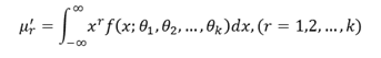
A parameter in statistics refers to an aspect of a population, as opposed to a statistic, which refers to an aspect, about a sample. For example, the population mean is a parameter, while the sample mean is a statistic. A parametric statistical test makes an assumption about the population parameters and the distributions that the data comes from. These types of tests assume to data is from normal distribution.

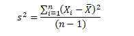
Data that is assumed to have been drawn from a particular distribution, and that is used in a parametric test.

Parametric equations are used in calculus to deal with the problems that arise when trying to find functions that describe curves. These equations are beyond the scope of this site, but you can find an excellent rundown of how to use these types of equations here.

The parametric tests are:
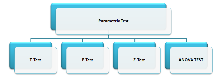
Let’s discuss about each test in details.
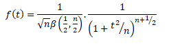
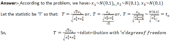
T-TEST

The T-test is one of, inferential statistics. It is used to determine whether there is a significant difference between the means of two groups or not. When the difference between two population averages is being investigated, a t-test is used. In other words, a t-test is used when we wish to compare two means. Essentially, a t-test allows us to compare the average values of the two data sets and determine if they came from the same population. In the above examples, if we were to take a sample of students from class A and another sample of students from class B, we would not expect them to have exactly the same mean and standard deviation.

Mathematically, the t-test takes a sample from each of the two sets and establishes the problem statement by assuming a null hypothesis that the two means are equal. Based on the applicable formulas, certain values are calculated and compared against the standard values, and the assumed null hypothesis is accepted or rejected accordingly.

If the null hypothesis qualifies to be rejected, it indicates that data readings are strong and are probably not due to chance. The t-test is just one of many tests used for this purpose. Statisticians must additionally use tests other than the t-test to examine more variables and tests with larger sample sizes. For a large sample size, statisticians use a z-test. Other testing options include the chi-square test and the f-test.

T-Test Assumptions

  • The first assumption made regarding t-tests concerns the scale of measurement. The assumption for a t-test is that the scale of measurement applied to the data collected follows a continuous or ordinal scale, such as the scores for an IQ test.
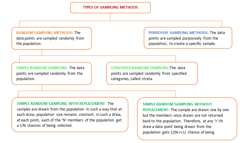
  • The second assumption made is that of a simple random sample, that the data is collected from a representative, randomly selected portion of the total population.
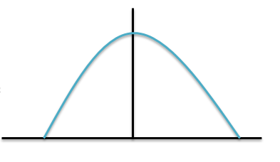
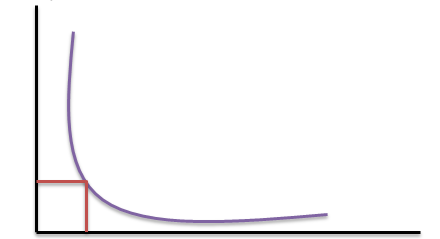
  • The third assumption is the data, when plotted, results in a normal distribution, bell-shaped distribution curve.
  • The final assumption is the homogeneity of variance. Homogeneous, or equal, variance exists when the standard deviations of samples are approximately equal.

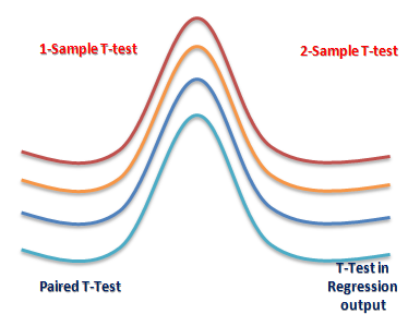
There are three types to T-test: (i) Correlated or paired T-test, (ii) Equal variance(or pooled) T-test (iii) Unequal variance T-test.

Z-TEST

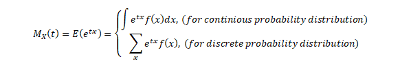
A z-test is a statistical test used to determine whether two population means are different when the variances are known and the sample size is large. The test statistic is assumed to have a normal distribution, and nuisance parameters such as standard deviation should be known in order for an accurate z-test to be performed. A z-statistic, or z-score, is a number representing how many standard deviations above or below the mean population a score derived from a z-test is.

The z-test is also a hypothesis test in which the z-statistic follows a normal distribution. The z-test is best used for greater-than-30 samples because, under the central limit theorem, as the number of samples gets larger, the samples are considered to be approximately normally distributed. When conducting a z-test, the null and alternative hypotheses, alpha and z-score should be stated. Next, the test statistic should be calculated, and the results and conclusion stated. Examples of tests that can be conducted as z-tests include a one-sample location test, a two-sample location test, a paired difference test, and a maximum likelihood estimate. Z-tests are closely related to t-tests, but t-tests are best performed when an experiment has a small sample size. Also, t-tests assume the standard deviation is unknown, while z-tests assume it is known. If the standard deviation of the population is unknown, the assumption of the sample variance equaling the population variance is made.

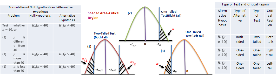
One Sample Z-test: A one sample z test is one of the most basic types of hypothesis test. In order to run a one sample z test, its work through several steps:

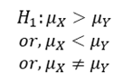
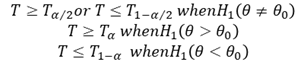
Step 1: Null hypothesis is one of the common stumbling blocks–in order to make sense of your sample and have the one sample z test give you the right information it must make sure written the null hypothesis and alternate hypothesis correctly. For example, you might be asked to test the hypothesis that the mean weight gain of an women was more than 30 pounds. Your null hypothesis would be: H0 : μ = 30 and your alternate hypothesis would be H, sub>1: μ > 30.

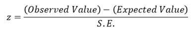
Step 2: Use the z-formula to find a z-score

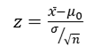
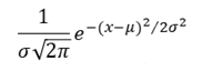
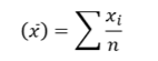
All you do is put in the values you are given into the formula. Your question should give you the sample mean (x̄), the standard deviation (σ), and the number of items in the sample (n). Your hypothesized mean (in other words, the mean you are testing the hypothesis for, or your null hypothesis) is μ0 .

Two Sample Z Test: The z-Test: Two- Sample for Means tool runs a two sample z-Test means with known variances to test the null hypothesis that there is no difference between the means of two independent populations. This tool can be used to run a one-sided or two-sided test z-test.

ANOVA

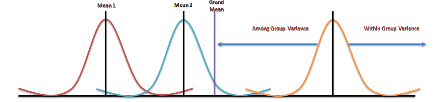
Analysis of variance (ANOVA) is an analysis tool used in statistics that splits an observed aggregate variability found inside a data set into two parts: systematic factors and random factors. The systematic factors have a statistical influence on the given data set, while the random factors do not. Analysts use the ANOVA test to determine the influence that independent variables have on the dependent variable in a regression study.
The ANOVA test is the initial step in analysing factors that affect a given data set. Once the test is finished, an analyst performs additional testing on the methodical factors that measurably contribute to the data set’s inconsistency. The analyst utilizes the ANOVA test results in an f-test to generate additional data that aligns with the proposed regression models. The ANOVA test allows a comparison of more than two groups at the same time to determine whether a relationship exists between them. The result of the ANOVA formula, the F statistic (also called the F-ratio), allows for the analysis of multiple groups of data to determine the variability between samples and within samples.

If no real difference exists between the tested groups, which is called the null hypothesis, the result of the ANOVA’s F-ratio statistic will be close to 1. Fluctuations in its sampling will likely follow the Fisher F distribution. This is actually a group of distribution functions, with two characteristic numbers, called the numerator degrees of freedom and the denominator degrees of freedom.

One-way Anova: A one-way ANOVA uses one independent variable, use a one-way ANOVA when collected data about one categorical independent variable and one quantitative dependent variable. The independent variable should have at least three levels (i.e. at least three different groups or categories). ANOVA that if the dependent variable changes according to the level of the independent variable.

Two-way Anova: A two-way ANOVA is used to estimate how the mean of a quantitative variable changes according to the levels of two categorical variables. Use a two-way ANOVA when you want to know how two independent variables, in combination, affect a dependent variable.
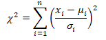
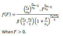
F-TEST

An “F Test” is a catch-all term for any test that uses the F-distribution. In most cases, when people talk about the F-Test, what they are actually talking about is The F-Test to compare two variances. However, the f-statistic is used in a variety of tests including regression analysis, the Chow test and the Scheffe Test (a post-hoc ANOVA test).

F Test to Compare Two Variances

 A Statistical F Test uses an F Statistic to compare two variances, s1 and s2 , by dividing them. The result is always a positive number (because variances are always positive). The equation for comparing two variances with the f-test is:

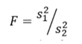
If the variances are equal, the ratio of the variances will equal 1. For example, if you had two data sets with a sample 1 (variance of 10) and a sample 2 (variance of 10), the ratio would be 10/10 = 1.

You always test that the population variances are equal when running an F Test. In other words, you always assume that the variances are equal to 1. Therefore, your null hypothesis will always be that the variances are equal.
Assumptions

Several assumptions are made for the test. Your population must be approximately normally distributed (i.e. fit the shape of a bell curve) in order to use the test. Plus, the samples must be independent events. In addition, you’ll want to bear in mind a few important points:

  1. The larger variance should always go in the numerator (the top number) to force the test into a right-tailed test. Right-tailed tests are easier to calculate.
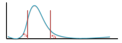
  2. For two-tailed tests, divide alpha by 2 before finding the right critical value.
  3. If you are given standard deviations, they must be squared to get the variances.
  4. If your degrees of freedom aren’t listed in the F Table, use the larger critical value. This helps to avoid the possibility of Type I errors.

CONCLUSION

Conventional statistical procedures may also call parametric tests. In every parametric test, for example, you have to use statistics to estimate the parameter of the population. Because of such estimation, you have to follow a process that includes a sample as well as a sampling distribution and a population along with certain parametric assumptions that required, which makes sure that all components compatible with one another.

 An example can use to explain this. Observations are first of all quite independent, the sample data doesn’t have any normal distributions and the scores in the different groups have some homogeneous variances. Parametric tests are based on the distribution, parametric statistical tests are only applicable to the variables. There’re no parametric tests that exist for the nominal scale date, and finally, they are quite powerful when they exist. There are mainly four types of Parametric Hypothesis Test which already mentioned in previous slides.

Advantages of Parametric Test

One of the biggest and best advantages of using parametric tests is first of all that you don’t need much data that could be converted in some order or format of ranks. The process of conversion is something that appears in rank format and to be able to use a parametric test regularly, you will end up with a severe loss in precision. Another big advantage of using parametric tests is the fact that you can calculate everything so easily. In short, you will be able to find software much quicker so that you can calculate them fast and quick. Apart from parametric tests, there are other non-parametric tests, where the distributors are quite different and they are not all that easy when it comes to testing such questions that focus related to the means and shapes of such distributions.

Disadvantages of Parametric Test

Parametric tests are not valid when it comes to small data sets. The requirement that the populations are not still valid on the small sets of data, the requirement that the populations which are under study have the same kind of variance and the need for such variables are being tested and have been measured at the same scale of intervals. Another disadvantage of parametric tests is that the size of the sample is always very big, something you will not find among non-parametric tests. That makes it a little difficult to carry out the whole test.

This particular discussion on parametric tests ends here, and at the end of this you must have developed clear ideas regarding these test categories. To find more such posts on Data Science training topics follow the Dexlab Analytics blog.


.

Basic of Statistical Inference Part-IV: An Overview of Hypothesis Testing

Basic of Statistical Inference Part-IV: An Overview of Hypothesis Testing

  1. Introduction
  2. What is Hypothesis Testing?
  3. Null Hypothesis, Alternative Hypothesis, Power of Test
  4. Type I and Type II Error
  5. Level of Significance, Critical Region
  6. Two-tailed and One-tailed test
  7. Solving Testing of Hypothesis Problem 8. Conclusion
  8. Conclusion

In this series we cover the basic of statistical inference, this is the fourth part of our discussion where we explain the concept of hypothesis testing which is a statistical technique. You could also check out the 3rd part of the series here.

Introduction

The objective of sampling is to study the features of the population on the basis of sample observations. A carefully selected sample is expected to reveal these features, and hence we shall infer about the population from a statistical analysis of the sample. This process is known as Statistical Inference.

 There are two types of problems. Firstly, we may have no information at all about some characteristics of the population, especially the values of the parameters involved in the distribution, and it is required to obtain estimates of these parameters. This is the problem of Estimation. Secondly, some information or hypothetical values of the parameters may be available, and it is required to test how far the hypothesis is tenable in the light of the information provided by the sample. This is the problem of Test of Hypothesis or Test of Significance.

 In many practical problems, statisticians are called upon to make decisions about a population on the basis of sample observations. For example, given a random sample, it may be required to decide whether the population, from which the sample has been obtained, is a normal distribution with mean = 40 and s.d. = 3 or not. In attempting to reach such decisions, it is necessary to make certain assumptions or guesses about the characteristics of population, particularly about the probability distribution or the values of its parameters. Such an assumption or statement about the population is called Statistical Hypothesis. The validity of a hypothesis will be tested by analyzing the sample. The procedure which enables us to decide whether a certain hypothesis is true or not, is called Test of Significance or Test of Hypothesis.

What Is Testing Of Hypothesis?

Statistical Hypothesis

Hypothesis is a statistical statement or a conjecture about the value of a parameter. The basic hypothesis being tested is called the null hypothesis. It is sometimes regarded as representing the current state of knowledge & belief about the value being tested. In a test the null hypothesis is constructed with alternative hypothesis denoted by 𝐻1 ,when a hypothesis is completely specified then it is called a simple hypothesis, when all factors of a distribution are not known then the hypothesis is known as a composite hypothesis.

Testing Of Hypothesis

The entire process of statistical inference is mainly inductive in nature, i.e., it is based on deciding the characteristics of the population on the basis of sample study. Such a decision always involves an element of risk i.e., the risk of taking wrong decisions. It is here that modern theory of probability plays a vital role & the statistical technique that helps us at arriving at the criterion for such decision is known as the testing of hypothesis.

Testing Of Statistical Hypothesis

A test of a statistical hypothesis is a two action decision after observing a random sample from the given population. The two action being the acceptance or rejection of hypothesis under consideration. Therefore a test is a rule which divides the entire sample space into two subsets.

  1. A region is which the data is consistent with 𝐻0.
  2. The second is its complement in which the data is inconsistent with 𝐻0.

The actual decision is however based on the values of the suitable functions of the data, the test statistic. The set of all possible values of a test statistic which is consistent with 𝐻0 is the acceptance region and all these values of the test statistic which is inconsistent with 𝐻0 is called the critical region. One important condition that must be kept in mind for efficient working of a test statistic is that the distribution must be specified.

Does the acceptance of a statistical hypothesis necessarily imply that it is true?

The truth a fallacy of a statistical hypothesis is based on the information contained in the sample. The rejection or the acceptance of the hypothesis is contingent on the consistency or inconsistency of the 𝐻0 with the sample observations. Therefore it should be clearly bowed in mind that the acceptance of a statistical hypothesis is due to the insufficient evidence provided by the sample to reject it & it doesn’t necessarily imply that it is true.

Elements: Null Hypothesis, Alternative Hypothesis, Pot

Null Hypothesis

A Null hypothesis is a hypothesis that says there is no statistical significance between the two variables in the hypothesis. There is no difference between certain characteristics of a population. It is denoted by the symbol 𝐻0. For example, the null hypothesis may be that the population mean is 40 then

 𝐻0(𝜇 = 40)

Let us suppose that two different concerns manufacture drugs for including sleep, drug A manufactured by first concern and drug B manufactured by second concern. Each company claims that its drug is superior to that of the other and it is desired to test which is a superior drug A or B? To formulate the statistical hypothesis let X be a random variable which denotes the additional hours of sleep gained by an individual when drug A is given and let the random variable Y denote the additional hours to sleep gained when drug B is used. Let us suppose that X and Y follow the probability distributions with means 𝜇𝑥 and 𝜇𝑌 respectively.

Here our null hypothesis would be that there is no difference between the effects of two drugs. Symbolically,

𝐻0: 𝜇𝑋 = 𝜇𝑌

Alternative Hypothesis

A statistical hypothesis which differs from the null hypothesis is called an Alternative Hypothesis, and is denoted by 𝐻1. The alternative hypothesis is not tested, but its acceptance (rejection) depends on the rejection (acceptance) of the null hypothesis. Alternative hypothesis contradicts the null hypothesis. The choice of an appropriate critical region depends on the type of alternative hypothesis, whether both-sided, one-sided (right/left) or specified alternative.

Alternative hypothesis is usually denoted by 𝐻1.

For example, in the drugs problem, the alternative hypothesis could be

Power Of Test

The null hypothesis 𝐻0 𝜃 = 𝜃0 is accepted when the observed value of test statistic lies the critical region, as determined by the test procedure. Suppose that the true value of 𝜃 is not 𝜃0, but another value 𝜃1, i.e. a specified alternative hypothesis 𝐻1 𝜃 = 𝜃1 is true. Type II error is committed if 𝐻0 is not rejected, i.e. the test statistic lies outside the critical region. Hence the probability of Type II error is a function of 𝜃1, because now 𝜃 = 𝜃1 is assumed to be true. If 𝛽 𝜃1 denotes the probability of Type II error, when 𝜃 = 𝜃1 is true, the complementary probability 1 − 𝛽 𝜃1 is called power of the test against the specified alternative 𝐻1 𝜃 = 𝜃1 . Power = 1-Probability of Type II error=Probability of rejection 𝐻0 when 𝐻1 is true Obviously, we could like a test to be as ‘powerful’ as possible for all critical regions of the same size. Treated as a function of 𝜃, the expression of 𝑃 𝜃 = 1 − 𝛽 𝜃 is called Power Function of the test for 𝜃0 against 𝜃. the curve obtained by plotting P(𝜃) against all possible values of 𝜃, is known as Power Curve.

Elements: Type I & Type II Error

Type I Error & Type Ii Error

The procedure of testing statistical hypothesis does not guarantee that all decisions are perfectly accurate. At times, the test may lead to erroneous conclusions. This is so, because the decision is taken on the basis of sample values, which are themselves fluctuating and depend purely on chance. The errors in statistical decisions are two types:

  1. Type I Error – This is the error committed by the test in rejecting a true null hypothesis.
  2. Type II Error – This is the error committed by the test in accepting a false null hypothesis.

Considering for the population mean is 40, i.e. 𝐻0 𝜇 = 40 , let us imagine that we have a random sample from a population whose mean is really 40. if we apply the test for 𝐻0 𝜇 = 40 , we might find that the values of test statistic lines in the critical region, thereby leading to the conclusion that the population mean is not 40; i.e. the test rejects the null hypothesis although it is true. We have thus committed what is known as “Type I error” or “Error of first kind”. On the other hand, suppose that we have a random sample from a population whose mean is known to different from 40, say 43. if we apply the test for 𝐻0 𝜇 = 40 , the value of the statistic may, by chance, lie in the acceptance region, leading to the conclusion that the mean may be 40; i.e. the test does not reject the null hypothesis 𝐻0 𝜇 = 40 , although it is false. This is again another form of incorrect decision, and the error thus committed is known as “Type II error” or “Error of second kind”.

Using sampling distribution of the test statistic, we can measure in advance the probabilities of committing the two types of error. Since the null hypothesis is rejected only when the test statistic falls in the critical region.

Probability of Type I error = Probability of rejecting 𝐻0 𝜃 = 𝜃0 , when it is true
= Probability that the test statistic lies in the critical region, assuming 𝜃 = 𝜃0.

The probability of Type I error must not exceed the level of significance (𝛼) of the test.

𝑃𝑟𝑜𝑏𝑎𝑏𝑖𝑙𝑖𝑡𝑦 𝑜𝑓 𝑇𝑦𝑝𝑒 𝐼 𝑒𝑟𝑟𝑜𝑟 ≤ 𝐿𝑒𝑣𝑒𝑙 𝑜𝑓 𝑆𝑖𝑔𝑛𝑖𝑓𝑖𝑐𝑎𝑛𝑐𝑒

The probability of Type II error assumes different values for different values of 𝜃 covered by the alternative hypothesis 𝐻1. Since the null hypothesis is accepted only when the observed value of the best statistic lies outside the critical region.

Probability of Type II error 𝑊ℎ𝑒𝑛 𝜃 = 𝜃1
= Probability of accepting 𝐻0 𝜃 = 𝜃0 , when it is false
= Probability that the test statistic lies in the region of acceptance, assuming 𝜃 = 𝜃1

The probability of Type I error is necessary for constructing a test of significance. It is in fact the ‘size of the Critical Region’. The probability of Type II error is used to measure the “power” of the test in detecting falsity of the null hypothesis. When the population has a continuous distribution

Probability of Type I error
= Level of significance
= Size of critical region

Elements: Level Of Significance & Critical Region

Level Of Significance And Critical Region

The decision about rejection or otherwise of the null hypothesis is based on probability considerations. Assuming the null hypothesis to be true, we calculate the probability of obtaining a difference equal to or greater than the observed difference. If this probability is found to be small, say less than .05, the conclusion is that the observed value of the statistic is rather unusual and has been caused due to the underlying assumption (i.e. null hypothesis) that is not true. We say that the observed difference is significant at 5 per cent level, and hence the ‘null hypothesis is rejected’ at 5 per cent level of significance. If, however, this probability is not very small, say more than .05, the observed difference cannot be considered to be unusual and is attributed to sampling fluctuation only. The difference is, now said to be not significant at 5 per cent level, and we conclude that there is no reason to reject the null hypothesis’ at 5 per cent level of significance. It has become customary to use 5% and 1% level of significance, although other levels, such as 2% or 5% may also be used.

Without actually going to calculate this probability, the test of significance may be simplified as follows. From the sampling distribution of the statistic, we find the maximum difference is which is exceeded in (say 5) percent of cases. If the observed difference in larger than this value, the null hypothesis is rejected. It is less there in no reason to reject the null hypothesis.

Suppose, the sampling distribution of the statistic is a normal distribution. Since the area under normal curve outside the ordinates at mean ±1.96 (𝑠. 𝑑. ) is only 5%, the probability that the observed value of the statistic differs from the expected value of 1.96 times the S.E. or more is .05; and the probability of a larger difference will be still smaller. If, therefore

Is either greater than 1.96 or less than -1.96 (i.e. numerically greater than 1.96), the null hypothesis 𝐻0 is rejected at 5% level of significance. The set values 𝑧 ≥ 1.96 𝑜𝑟 ≤ −1.96, i.e.

|𝑧| ≥ 1.96

constitutes what is called the Critical Region for the test. Similarly since the area outside mean ±2.58 (s.d.) is only 1%. 𝐻0 is rejected at 1% level of significance, if z numerically exceeds 258, i.e. the critical region is 𝑧 ≥ 2.58 at 1% level. Using the sampling distribution of an appropriate test statistic we are able to establish the maximum difference at a specified level between the observed and expected values that is consistent with null hypothesis 𝐻0 . The set of values of the test statistic corresponding to this difference which lead to the acceptance of 𝐻0 is called Region of acceptance. Conversely, the set of values of the statistic leading to the rejection of 𝐻0 is referred to as Region of Rejection or “Critical Region” of the test. The value of the statistic which lies at the boundary of the regions of acceptance and the rejection is called Critical value. When the null hypothesis is true, the probability of observed value of the test statistic falling in the critical region is often called the “Size of Critical Region”.

𝑆𝑖𝑧𝑒 𝑜𝑓 𝐶𝑟𝑖𝑡𝑖𝑐𝑎𝑙 𝑅𝑒𝑔𝑖𝑜𝑛 ≤ 𝐿𝑒𝑣𝑒𝑙 𝑜𝑓 𝑆𝑖𝑔𝑛𝑖𝑓𝑖𝑐𝑎𝑛𝑐𝑒

However, for a continuous population, the critical region is so determined that its size equals the Level of Significance (𝛼).

Two-Tailed And One-Tailed Tests

Our discussion above were centered around testing the significance of ‘difference’ between the observed and expected values, i.e. whether the observed value is significantly different from (i.e. either larger or smaller than) the expected value, as could arise due to fluctuations of random sampling. In the illustration, the null hypothesis is tested against “both-sided alternatives” 𝜇 > 40 𝑜𝑟 𝜇 < 40 , i.e.

𝐻0 𝜇 = 40 𝑎𝑔𝑎𝑖𝑛𝑠𝑡 𝐻1 𝜇 ≠ 40

Thus assuming 𝐻0 to be true, we would be looking for large differences on both sides of the expected value, i.e. in “both tails” of the distribution. Such tests are, therefore, called “Two-tailed tests”.

Sometimes we are interested in tests for large differences on one side only i.e., in one ‘one tail’ of the distribution. For example, whether a change in the production bricks with a ‘higher’ breaking strength, or whether a change in the production technique yields ‘lower’ percentage of defectives. These are known as “One-tailed tests”.

For testing the null hypothesis against “one-sided alternatives (right side)” 𝜇 > 40 , i.e.

𝐻0 𝜇 = 40 𝑎𝑔𝑎𝑖𝑛𝑠𝑡𝐻1 𝜇 > 40

The calculated value of the statistic z is compared with 1.645, since 5% of the area under the standard normal curve lies to the right of 1.645. if the observed value of z exceeds 1.645, the null hypothesis 𝐻0 is rejected at 5% level of significance. If a 1% level were used, we would replace 1.645 by 2.33. thus the critical regions for test at 5% and 1% levels are 𝑧 ≥ 1.645 and 𝑧 ≥ 2.33 respectively.

For testing the null hypothesis against “one-sided alternatives (left side)” 𝜇 < 40 i.e.

𝐻0 𝜇 = 40 𝑎𝑔𝑎𝑖𝑛𝑠𝑡𝐻1 𝜇 < 40

The value of z is compared with -1.645 for significance at 5% level, and with -2.33 for significance at 1% level. The critical regions are now 𝑧 ≤ −1.645 and 𝑧 ≤ −2.33 for 5% and 1% levels respectively. In fact, the sampling distributions of many of the commonly-used statistics can be approximated by normal distributions as the sample size increases, so that these rules are applicable in most cases when the sample size is ‘large’, say, more than 30. It is evident that the same null hypothesis may be tested against alternative hypothesis of different types depending on the nature of the problem. Correspondingly, the type of test and the critical region associated with each test will also be different.

Solving Testing Of Hypothesis Problem

Step 1
Set up the “Null Hypothesis” 𝐻0 and the “Alternative Hypothesis” 𝐻1 on the basis of the given problem. The null hypothesis usually specifies the values of some parameters involved in the population: 𝐻0 𝜃 = 𝜃0 . The alternative hypothesis may be any one of the following types: 𝐻1 ( ) 𝜃 ≠ 𝜃1 𝐻1 𝜃 > 𝜃0 , 𝐻1 𝜃 < 𝜃0 . The types of alternative hypothesis determines whether to use a two-tailed or one-tailed test (right or left tail).

Step 2

State the appropriate “test statistic” T and also its sampling distribution, when the null hypothesis is true. In large sample tests the statistic 𝑧 = (𝑇 − 𝜃0)Τ𝑆. 𝐸. , (T) which approximately follows Standard Normal Distribution, is often used. In small sample tests, the population is assumed to be Normal and various test statistics are used which follow Standard Normal, Chi-square, t for F distribution exactly.

Step 3
Select the “level of significance” 𝛼 of the test, if it is not specified in the given problem. This represents the maximum probability of committing a Type I error, i.e., of making a wrong decision by the test procedure when in fact the null hypothesis is true. Usually, a 5% or 1% level of significance is used (If nothing is mentioned, use 5% level).

Step 4

Find the “Critical region” of the test at the chosen level of significance. This represents the set of values of the test statistic which lead to rejection of the null hypothesis. The critical region always appears in one or both tails of the distribution, depending on weather the alternative hypothesis is one-sided or both-sided. The area in the tails must be equal to the level of significance 𝛼. For a one-tailed test, 𝛼 appears in one tail and for two-tailed test 𝛼/2 appears in each tail of the distribution. The critical region is

Where 𝑇𝛼 is the value of T such that the area to its tight is 𝛼.

Step 5

Compute the value of the test statistic T on the basis of sample data the null hypothesis. In large sample tests, if some parameters remain unknown they should be estimated from the sample.
Step 6

If the computed value of test statistic T lies in the critical region, “reject 𝐻0”; otherwise “do not reject 𝐻0 ”. The decision regarding rejection or otherwise of 𝐻0 is made after a comparison of the computed value of T with critical value (i.e., boundary value of the appropriate critical region).

Step 7
Write the conclusion in plain non-technical language. If 𝐻0 is rejected, the interpretation is: “the data are not consistent with the assumption that the null hypothesis is true and hence 𝐻0 is not tenable”. If 𝐻0 is not rejected, “the data cannot provide any evidence against the null hypothesis and hence 𝐻0 may be accepted to the true”. The conclusion should preferably be given in the words stated in the problem.

Conclusion

Hypothesis is a statistical statement or a conjecture about the value of a parameter. The legal concept that one is innocent until proven guilty has an analogous use in the world of statistics. In devising a test, statisticians do not attempt to prove that a particular statement or hypothesis is true. Instead, they assume that the hypothesis is incorrect (like not guilty), and then work to find statistical evidence that would allow them to overturn that assumption. In statistics this process is referred to as hypothesis testing, and it is often used to test the relationship between two variables. A hypothesis makes a prediction about some relationship of interest. Then, based on actual data and a pre-selected level of statistical significance, that hypothesis is either accepted or rejected. There are some elements of hypothesis like null hypothesis, alternative hypothesis, type I & type II error, level of significance, critical region and power of test and some processes like one and two tail test to find the critical region of the graph as well as the error that help us reach the final conclusion.

A Null hypothesis is a hypothesis that says there is no statistical significance between the two variables in the hypothesis. There is no difference between certain characteristics of a population. It is denoted by the symbol 𝐻0. A statistical hypothesis which differs from the null hypothesis is called an Alternative Hypothesis, and is denoted by 𝐻1. The procedure of testing statistical hypothesis does not guarantee that all decisions are perfectly accurate. At times, the test may lead to erroneous conclusions. This is so, because the decision is taken on the basis of sample values, which are themselves fluctuating and depend purely on chance, this process called types of error. Hypothesis testing is very important part of statistical analysis. By the help of hypothesis testing many business problem can be solved accurately.

That was the fourth part of the series, that explained hypothesis testing and hopefully it clarified your notion of the same by discussing each crucial aspect of it. You can find more informative posts like this one on Data Science course topics. Just keep on following the Dexlab Analytics blog to stay informed.


.


Basic of Statistical Inference: An Introduction to the Theory of Estimation (Part-III)

Basic of Statistical Inference: An Introduction to the Theory of Estimation (Part-III)

As we continue our discussion on statistical inference, we move on to the estimation theory. Here you will learn about the concept of estimation, along with different elements and methods of estimation. You can check part-II here.

Content:

  1. Introduction
  2. Element of Estimation (Parameter, Statistic, Relation between Statistic and Parameter
  3. What is Estimation (Point estimation, Interval estimation)
  4. Characteristics of Estimation (Unbiasedness)
  5. Characteristics of Estimation (Sufficiency, Efficiency, Consistency)
  6. Method of Estimation (MLE, MLS)
  7. Method of Estimation (MMV, MM)
  8. Conclusion

Introduction

The estimation is the process of providing numerical values of the unknown parameter to the population. There are mainly two types of estimation process Point estimation and Interval estimation and confidence interval is the part of the interval estimation. We will also discuss about the elements of the estimation like parameter, statistic and estimator.

The characteristics of estimators are – (i) Unbiasedness – This is desirable property of a good estimator. (ii) Consistency – An estimator is said to be consistent if increasing the sample size produces an estimate with smaller standard error. (iii) Efficiency – An estimator should be an efficient estimator. (iv) Sufficiency – An estimator is said to be sufficient for a parameter, if it contains all the information in the sample regarding the parameter.

The methods of estimation are– (i) Method of maximum likelihood, (ii) Method of least square, (iii) Method of minimum variance, (iv) Method of moments.

Element For Estimation

Parameter

Parameter is an unknown numerical factor of the population. The primary interest of any survey lies in knowing the values of different measures of the population distribution of a variable of interest. The measures of population distribution involves its mean, standard deviation etc. which is calculated on the basis of the population values of the variable. In other words, the parameter is a functional form of all the population unit.

Statistic

Any statistical measure calculated on the basis of sample observations is called Statistic. Like sample mean, sample standard deviation, etc. Sample statistic are always known to us.

Estimator An estimator is a measure computed on the basis of sample values. It is a functional from of all sample observe prorating a representative value of the collected sample. Relation Between Parameter And Statistic

Parameter is a fixed measure describing the whole population (population being a group of people, things, animals, phenomena that share common characteristics.) A statistic is a characteristic of a sample, a portion of the target population. A parameter is fixed, unknown numerical value, while the statistic is a known number and a variable which depends on the portion of the population. Sample statistic and population parameters have different statistical notations: In population parameter, population proportion is represented by P, mean is represented by µ (Greek letter mu), σ2 represents variance, N represents population size, σ (Greek letter sigma) represents standard deviation, σx̄ represents Standard error of mean, σ/µ represents Coefficient of variation, (X-µ)/σ represents standardized variate (z), and σp represents standard error of proportion.

In sample statistics, mean is represented by x̄(x-bar), sample proportion is represented by p̂(p-hat), s represents standard deviation, s2 represents variance, sample size is represented by n, sx̄ represents Standard error of mean, sp represents standard error of proportion, s/(x̄) represents Coefficient of variation, and (x-x)/s ̄ represents standardized variate (z).

What Is Estimation?

Estimation refers to the process by which one makes an idea about a population, based on information obtained from a sample.

Suppose we have a random sample 𝑥1, 𝑥2, … , 𝑥𝑛 on a variable x, whose distribution in the population involves an unknown parameter 𝜃. It is required to find an estimate of 𝜃 on the basis of sample values. The estimation is done in two different ways: (i) Point Estimation, and (ii) Interval Estimation.

In point estimation, the estimated value is given by a single quantity, which is a function of sample observations. This function is called the ‘estimator’ of the parameter, and the value of the estimator in a particular sample is called an ‘estimate’.

Interval estimation, an interval within which the parameter is expected to lie in given by using two quantities based on sample values. This is known as Confidence interval, and the two quantities which are used to specify the interval, are known as Confidence Limits.

 
Point Estimation

Many functions of sample observations may be proposed as estimators of the same parameter. For example, either the mean or median or mode of the sample values may be used to estimate the parameter 𝜇 of the normal distribution with probability density function

Which we shall in future refer to as 𝑁(𝜇, 𝜎 2 ).

Interval Estimation

In statistical analysis it is not always possible to find out an exact point estimate to form an idea about the population parameters. An approximately true picture can be formed if the sample estimations satisfy some important property such as unbiasedness consistency, sufficiency, efficiency & so on. So, a more general concept of estimation would be to find out an interval based on sample values which is expected to include the unknown parameter with a specified probability. This is known as the theory of interval estimator.

Confidence Interval

Let 𝑥1, 𝑥2,… , 𝑥𝑛 be a random sample from a population involve an unknown parameter 𝜃. Our job is to find out two functions 𝑡1 & 𝑡2 of the sample values. Such that the probability of 𝜃 being included in the random interval 𝑡1,𝑡2 has a given value say 1 − 𝛼 . So,

Here the interval [𝑡1,𝑡2] is called a 100 × ( ) 1 − 𝛼 % confidence interval for the parameter 𝜃. The quantities 𝑡1 & 𝑡2 which serve as the lower & upper limits of the interval are known as confidence limits. 1 − 𝛼 is called the confidence coefficient. The is a sort of measures of the trust or confidence that one may place in the interval for actually including 𝜃.

Characteristics of Estimation

Unbiasedness

A statistic t is said to be an Unbiased Estimator of parameter 𝜃, if the expected value of t is 𝜃. 𝐸 𝑡 = 𝜃 Otherwise, the estimator is said to be ‘biased’. The bias of a statistic in estimating 𝜃 is given as 𝐵𝑖𝑎𝑠 = 𝐸 𝑡 − 𝜃 Let 𝑥1, 𝑥2,… , 𝑥𝑛 be a random sample drawn from a population with mean 𝜇 and variance 𝜎 2 . Then Sample mean

Sample varianceThe sample mean 𝑥ҧis an unbiased estimator of the population mean 𝜇; because 𝐸 𝑥ҧ = 𝜇 The sample variance 𝑆 2 is a biased estimator of the population variance 𝜎 2 ; because  

An unbiased estimator of the population variance 𝜎 2 is given by

Because

The distinction between 𝑆 2 and 𝑠 2 in which only he denominators are different. 𝑆 2 is the variance of the sample observations, but 𝑠 2 is the ‘unbiased estimator’ of the variance (𝜎 2 ) in the population.

Example:

Characteristics of Estimation (Sufficiency, Efficiency, Consistency)

Consistency

A desirable property of good estimator is that its accuracy should increase when the sample becomes larger. That is, the estimator is expected to come closer to the parameter as the size of the sample increases.

A statistic 𝑡𝑛 computed from a sample of n observations is said to be a Consistent Estimator of a parameter 𝜃, if it converges in probability to 𝜃 as n tends to infinity. This means that the larger the sample size (n), the less is the chance that the difference between 𝑡𝑛 and 𝜃 will exceed any fixed value. In symbols, given any arbitrary small positive quantity 𝜖, 𝜇 , then the statistic 𝑡𝑛 will be a ‘consistent estimator’ of 𝜃. Consistency is a limiting property. Moreover, several consistent estimators may exist for the same parameter. For example, in sampling from a normal population 𝑁 𝜇, 𝜎 2 , both the sample mean and sample median are consistent estimators of 𝜇.

Efficiency

If we confine ourselves to unbiased estimates, there will, in general, exist more than one consistent estimator of a parameter. For example, in sampling from a normal population 𝑁 𝜇, 𝜎 2 , when 𝜎 2 is known, sample mean 𝑥ҧis an unbiased and consistent estimator of 𝜇. From symmetry it follows immediately the sample median (Md) is an unbiased estimate of 𝜇. Which is same as the population median. Also for large n,

Median is also an unbiased and consistent estimator of 𝜇.

Thus, there is necessity of some further criterion which will enable us to choose between the estimators with the common property of consistency.

Such a criterion which is based on the variance of the sampling distribution of estimators is usually known as Efficiency.

Sufficiency

A statistic is said to be a ‘sufficient estimator’ of a parameter 𝜃, if it contains all information in the sample about 𝜃. If a statistic t exists such that the joint distribution of the sample is expressible as the product of two factors, one of which is the sampling distribution of t and contains 𝜃, but the other factor is independent of 𝜃, then t will be a sufficient estimator of 𝜃.

Thus if 𝑥1, 𝑥2,… , 𝑥𝑛 is a random sample from a population whose probability mass function or probability density function is 𝑓 𝑥, 𝜃 , and t is a sufficient estimator of 𝜃 then we can write

Where g(t, 𝜃) is the sampling distribution of t and contains 𝜃, but ℎ (𝑥1, 𝑥2,… , 𝑥𝑛) is independent of 𝜃.

Since the parameter 𝜃 is occurring in the joint distribution of all the sample observations can be contained in the distribution of the statistic t, it is said that t alone can provide all ‘information’ about 𝜃 and is therefore “sufficient” for 𝜃.

Sufficient estimators are the most desirable kind of estimators, but unfortunately they exist in only relatively few cases. If a sufficient estimator exists, it can be found by the method of maximum likelihood.

In random sampling from a Normal population 𝑁 (𝜇, 𝜎 2) , the sample mean 𝑥ҧis a sufficient estimator of 𝜇.

Methods of Estimation (MLE, MLS)

Method of Maximum Likelihood

This is a convenient method for finding an estimator which satisfies most of the criteria discussed earlier. Let 𝑥1, 𝑥2,… , 𝑥𝑛 be a random sample from a population with p.m.f (for discrete case) or p.d.f. (for continuous case) 𝑓 𝑥, 𝜃 , where 𝜃 is the parameter. Then the joint distribution of the sample observations

is called the Likelihood Function of the sample. The Method of Maximum Likelihood consists in choosing as an estimator of 𝜃 that statistic, which when substituted for 𝜃, maximizes the likelihood function L. such a statistic is called a maximum likelihood estimator (m.l.e.). We shall denote the m.l.e. of 𝜃 by the symbol 𝜃0. Since log 𝐿 is maximum when L is maximum, in practice the m.l.e. of 𝜃 is obtained by maximizing log 𝐿 . This is achieved by differentiating log 𝐿 partially with respect to 𝜃, and using the two relations

The m.l.e. is not necessarily unbiased. But when the m.l.e. is biased, by a slight modification, it can be converted into an unbiased estimator. The m.l.e. tends to be distributed normally for large samples. The m.l.e. is invariant under functional transformations. If T is an m.l.e. of 𝜃, and 𝑔(𝜃) is a function of 𝜃, then g(T) is the m.l.e. of 𝑔(𝜃) .

Method Of Least Square

Method of Least Squares is a device for finding the equation of a specified type of curve, which best fits a given set of observations. The principal of least squares is used to fit a curve of the form:

𝑦𝑖 = 𝑓 𝑥𝑖 be a function where 𝑥𝑖 is an explanatory variable. & 𝑦𝑖 is the dependent variable. Let us assume a linear relationship between the dependent & independent variable. So,

𝑌𝑖 = 𝛼 + 𝛽𝑥𝑖 + 𝑒𝑖 ; 𝛼 = 𝑖𝑛𝑡𝑒𝑟𝑐𝑒𝑝𝑡 𝑓𝑜𝑟𝑚 𝛽 = 𝑅𝑒𝑠𝑝𝑜𝑛𝑠𝑖𝑣𝑒𝑛𝑒𝑠𝑠 𝑜𝑓 𝑌𝑖 𝑒𝑖 = 𝐸𝑟𝑟𝑜𝑟 𝑓𝑜𝑟𝑚

The objective of the researcher is to minimize σ𝑙𝑖 2, σ 𝑒𝑖 is not minimized because σ 𝑒𝑖 = 0 but actual error of individual observation can remain

The method of least squares can be used to fit other types of curves, e.g. parabola, exponential curve, etc. method of least squares is applied to find regression lines and also in the determination of trend in time series.

Methods of Estimation (MMV, MM)

Method of Minimum Variance

Minimum Variance Unbiased Estimates, the estimates 𝑖 𝑇 𝑖𝑠 𝑢𝑛𝑏𝑖𝑎𝑠𝑒𝑑 𝑓𝑜𝑟 𝛾 𝜃 , 𝑓𝑜𝑟 𝑎𝑙𝑙 𝜃𝜖𝜗 are unbiased and [(ii) It has smallest variance among the class of all unbiased estimators of 𝛾(𝜃), then T is called the minimum variance unbiased estimator (MVUE) of 𝛾(𝜃)] have minimum variance.

If 𝐿 = ς𝑖=1 𝑛 𝑓 𝑥𝑖 , 𝜃 , is the likelihood function of a random sample of n observations 𝑥1, 𝑥2, … , 𝑥𝑛 from a population with probability function 𝑓(𝑥, 𝜃), then the problem is to find a statistics 𝑡 = 𝑡(𝑥1, 𝑥2,… , 𝑥𝑛), such that

Method of Moments

This method was discovered and studied in detail by Karl Pearson. Let 𝑓 𝑥; 𝜃1, 𝜃2, … , 𝜃𝑘 be the density function of the parent population with k parameters 𝜃1, 𝜃2,… , 𝜃𝑘. If 𝜇𝑟 ′ denoted the rth moment about origin, then

Let 𝑥𝑖 , 𝑖 = 1,2, … , 𝑛 be a random sample of size n from the given population. The method of moments consists in solving the k-equations for 𝜃1, 𝜃2,… , 𝜃𝑘 in terms of 𝜇1 ′ , 𝜇2 ′ ,… , 𝜇𝑘 ′ and then replacing these moments 𝜇𝑟 ′ ; 𝑟 = 1,2,… , 𝑘 by the sample moments,

Where 𝑚𝑖 ′ is the ith moment about origin in the sample.

Then by the method of moments 𝜃1, 𝜃2,… , 𝜃𝑘 are the required estimator of 𝜃1, 𝜃2,… . , 𝜃𝑘 respectively.

Conclusion

Estimation theory is a branch of statistics and signal processing that deals with estimating the values of parameters based on measured/empirical data that has a random component. The parameters describe an unknown numerical factor of the population. The primary interest of any survey lies in knowing the values of different measures of the population distribution of a variable of interest. The measures of population distribution involves its mean, standard deviation etc. which is calculated on the basis of the population values of the variable. The estimation theory has its own characteristics like the data should be unbiased, a good estimator is that its accuracy should increase when the sample size becomes larger, The sample mean and sample median should be consistent estimators of parameter mean, The estimator is expected to come closer to the parameter as the size of the sample increases. Two consistent estimators for the same parameter, the statistic with the smaller sampling variance is said to be more efficient, so, efficiency is another characteristic of the estimation. The estimator should be sufficient estimator of a parameter theta.

The estimation theory follows some methods by this method and with the characteristics we can properly estimate from the data. The methods we already discussed that maximum likelihood method, least square method, minimum variance method & method of moments.

In real life, estimation is part of our everyday experience. When you’re shopping in the grocery store and trying to stay within a budget, for example, you estimate the cost of the items you put in your cart to keep a running total in your head. When you’re purchasing tickets for a group of people or splitting the cost of dinner between 8 friends, we estimate for ease. In many other field we can use the estimation theory specially for statistical analysis.

If you found this blog helpful then, then keep on exploring DexLab Analytics blog to pursue more informative posts on diverse topics such as python for data analysis. Also, check out part-I AND part- II of the series to keep pace.


.


Classical Inferential Statistics: Theory of Sampling (Part -II)

Classical Inferential Statistics: Theory of Sampling (Part -II)

Here is taking an in-depth look at how sampling distribution works along with a discussion on various types of the sampling distribution. This is a continuation of the discussion on Classical Inferential Statistics that focused on the theory of sampling, breaking it down to building blocks of classical sampling theory along with various kinds of sampling. You can read part 1 of the article here

Contents:

  1. Introduction
  2. Probability Density Function, Moment Generating Function, Sampling Distribution, Degrees of Freedom
  3. Gamma Function, Beta Function, Relation between Gamma & Beta Function
  4. Gamma Distribution
  5. Beta Distribution
  6. Chi-square Distribution & Exponential Distribution
  7. T-Distribution & F-Distribution

1. Introduction

The sampling distribution is a probability distribution of statistics obtained from a large number of samples drawn from a specific population. And the types of sampling distribution are- (i) Gamma Distribution, (ii) Beta Distribution, (iii) Chi-Square Distribution, (iv) Exponential Distribution, (v) T-Distribution & (vi) F-Distribution.

The key components for describing all these distributions are – (i) Probability Density Function – Which is the function whose integral is to be calculated to find probabilities associated with a continuous random variable and their shape(graph) for the same, (ii) Moment Generating Function – which helps to find the moment of those distributions, and (iii) Degrees of Freedom – It refers to the number of independent sample points and compute a static minus the number of parameters explained from the sample.

For Gamma and Beta distribution, we will discuss gamma and beta function and relation between them etc.

2. Probability Density Function, Moment Generating Function, Sampling Distribution, Degrees of Freedom

PROBABILITY DENSITY FUNCTION

Probability density function (PDF), in statistics, is a function whose integral is calculated to find probabilities associated with a continuous random variable (see continuity; probability theory). Its graph is a curve above the horizontal axis that defines a total area, between itself and the axis, of 1. The percentage of this area included between any two values coincides with the probability that the outcome of an observation described by the probability density function falls between those values. Every random variable is associated with a probability density function (e.g., a variable with a normal distribution is described by a bell curve). If X be continuous Random variable taking any continuous real values then f(x) is a probability density function if:-

Moment Generating Function

The moment generating function (m.g.f.) of a random variable X (about origin) having the probability function f(x) is given by:

The integration of summation being extended to the entire range of x, t being the real parameter and it is being assumed that the right-hand side of the equation is absolutely convergent for some positive number h such that –h<t<h.

SAMPLING DISTRIBUTION

It may be defined as the probability law which the statistic follows if repeated random samples of a fixed size are drawn from a specified population. A number of samples, each of size n, are taken from the same population and if for each sample the values of the statistic are calculated, a series of values of the statistic will be obtained. If the number of samples is large, these may be arranged into a frequency table. The frequency distribution of the statistic that would be obtained if the number of samples, each of the same size (say n), were infinite is called the Sampling distribution of the statistic

DEGREES OF FREEDOM

The term degrees of freedom (df) refers to the number of independent sample points used to compute a statistic minus the number of parameters estimated from the sample points: For example, consider the sample estimate of the population variance (s2)

Where is the score for observation i in the sample, X ̅ is the sample estimate of the population mean, n is the number of observation in the sample. The formula is based on n independent sample points and one estimated population parameter (x ̅). Therefore, the number of degrees of freedom is n minus one. For this example

df=n-1 

3. Gamma Function, Beta Function, Relation between Gamma &Beta Function

GAMMA FUNCTION

The Gamma function is defined for x>0 in integral form by the improper integral known as Euler’s integral of the second kind.

Many probability distributions are defined by using the gamma function, such as gamma distribution, beta distribution, chi-squared distribution, student’s t-distribution, etc. For data scientists, machine learning engineers, researchers, the Gamma function is probably one of the most widely used functions because it is employed in many distributions.

BETA FUNCTION

The Beta function is a function of two variables that is often found in probability theory and mathematical statistics.

The Beta function is a function B: R_(++)^2→R defined as follows:

There is also a Euler’s integral of the first kind.

For example, as a normalizing constant in the probability density functions of the F distribution and of the Student’s t distribution

RELATION BETWEEN GAMMA AND BETA FUNCTION

In the realm of Calculus, many complex integrals can be reduced to expressions involving the Beta Function. The Beta Function is important in calculus due to its close connection to the Gamma Function which is itself a generalization of the factorial function.

We know,

So, the product of two factorials as

Now apply the changes of variables t=xy and s=x(1-y) to this double integral. Note that t + s = x and that 0 < t < ∞ and 0 < x < ∞ and 0 < y < 1. The jacobian of this transformation is 


Since x > 0 we conclude that  Hence we have

Therefore,

4. Gamma Distribution

The gamma distribution is a widely used distribution. It is a right-skewed probability distribution. These distributions are useful in real life where something has a natural minimum of 0.

If X be a continuous random variable taking only positive values, then X is said to be following a gamma distribution iff its p.d.f can be expressed as:-

=0 otherwise….(1)


  • Probability Density Function for Gamma Distribution

For (1), to be the Probability Density Function, we must have:-

Now, f(x)>0 if  x>0 & f(x)=0 if x taking any non-positive values, so, f(x)≥0 ∀x .

Hence, condition (i) is satisfied. Now,

Using (3) & (4) in (2) we get:-

Hence, f(x) statistics condition (ii).

So,  equation  (1) is a proper pdf.

  • Moment Generating Function for Gamma Distribution

Moment generating functions are general procedure of finding out moments of a probability distribution mathematically it may be expressed as- M_x (t)=E(e^xt )

This represents raw moments of the random variable X about to the origin 0.

Three important properties of m.g.f. are:- (i)  where c is a constant.(ii) If ’s are independent Random variables i.e.  then   (iii) If X and Y are two random variables and if  then X and Y are two identical distribution this is called the uniqueness property,Calculating the m.g.f. of gamma distribution:

Using (2) and (3) in (1) we get:

5. Beta Distribution

In probability theory and statistics, the beta distribution is a family of continuous probability distributions defined on the interval [0, 1] parameterized by two positive shape parameters, denoted by α and β, that appear as exponents of the random variable and control the shape of the distribution.

The beta distribution has been applied to model the behavior of random variables limited to intervals of finite length in a wide variety of disciplines.

  • Probability Density Function for Beta Distribution

The probability density function (PDF) of the beta distribution, for 0 ≤ x ≤ 1, and shape parameters αβ > 0, is a power function of the variable x and of its reflection (1 − x) as follows:

Where Γ(z) is the gamma function. The beta function, B,  =+is a normalization constant to ensure that the total probability integrates to 1. In the above equations, x is a realization—an observed value that actually occurred—of a random process X.

This definition includes both ends x = 0 and x = 1, which is consistent with the definitions for other continuous distributions supported on a bounded interval which are special cases of the beta distribution, for example, the arcsine distribution, and consistent with several authors, like N. L. Johnson and S. Kotz. However, the inclusion of x= 0 and x= 1 does not work for αβ < 1; accordingly, several other authors, including W. Feller, choose to exclude the ends x = 0 and x = 1, (so that the two ends are not actually part of the domain of the density function) and consider instead 0 < x < 1. Several authors, including N. L. Johnson and S. Kotz, use the symbols p and q (instead of α and β) for the shape parameters of the beta distribution, reminiscent of the symbols are traditionally used for the parameters of the Bernoulli distribution, because the beta distribution approaches the Bernoulli distribution in the limit when both shape parameters α and β approach the value of zero.

In the following, a random variable X beta-distributed with parameters α and β will be denoted by:

Other notations for beta-distributed random variables used in the statistical literature are. X- Be(α,β)and X~β_(α,β)

  • Moment Generating Function for Beta Distribution


  • 6. Chi-square Distribution & Exponential Distribution

    CHI-SQUARE DISTRIBUTION

    A chi-square distribution is defined as the sum of the squares of standard normal variates. Let x be a random variable which follows normal distribution with mean μ& variance then standard normal variate is defined as: –

    The variate Z is said to follow a standard normal distribution with mean 0 and variance 1. Let X be a random variable containing observations,.

    Then the chi-square distribution is defined as:- So we can say:-

    A chi-square distribution with ‘n’ degree of freedom, where degrees of freedom refer to number of independent associations among variables.

    • The Probability Density Function of a Chi-Square Distribution:


    • The Moment Generating Function of Chi-Square Distribution:

    (4) is a required m.g.f. of the chi-square distribution.

    EXPONENTIAL DISTRIBUTION

    The Exponential distribution is one of the widely used continuous distributions. It is often used to model the time elapsed between events.

    • The Probability Density Function of Exponential Distribution:

    Let X be a continuous random variable assuming only real values then X is said to be following an exponential distribution iff:-

    Therefore, exponential distribution is a special case of gamma

    distribution with v = 1.

    • The Moment Generating Function of Exponential Distribution:

    Let X~Exponential (λ), we can find its expected value as follows, using integration by parts:


    Now let’s find Var (X), we have

    7. T-Distribution & F-Distribution

    T-DISTRIBUTION

    • Student’s t-distribution:

    If x1,x2,… ,xn be ‘n’ random samples drawn from a normal population having mean & standard deviation  then the statistics following student t-distribution with (n-1) degrees of freedom.

    • Fisher’s t-distribution:

    Let X~N(0,1) & let the random variable Y~X_n^2. Both X & Y are independent random variables. Then the fisher’s t-distribution is defined as :-


    • Probability Density Function for t-distribution:

    Where, t2 > 0 Where, v=(n-1) degrees of freedom

                    = 0    , otherwise

    For Fisher’s t-distribution:

    Where, t2 > 0

    =0 otherwise

    • Application of t-distribution:

    If  x1,x2, and x3 are independent random variables. Each following a standard normal distribution. What will be the distribution of  


    F- DISTRUBUTION

    The F-Distribution is a ration of two chi-square distributions. If X be a random variable which follows a fisher’s t-distribution.Then:-

    Squaring the above expression we get:

    The R.V. X2~F1, n. Then we say X2 follows F-distribution with 1,n degrees of freedom.

    • Probability Density Function for F-distribution:

    • Application of F-Distribution:

    Let x1,x2,… ,xn be a random sample drawn from a normal population with mean μ & variance σ2. where both μ & σ are unknown. Obtain the MLEs of θ.

    Let x1,x2,… ,xn be ‘n’ random sample drawn from a normal population with mean μ & variance σ2.

    Taking logarithms on both sides; we get:-

    CONCLUSION: That was a thorough analysis of different types of sampling distribution along with their distinct functions and interrelations. If the resource was useful in understanding statistical analytics, find more such informative and analytical, subject-oriented discussion regarding statistical analytics courses on DexLab Analytics blog.


    .

  • Classical Inferential Statistics: Theory of Sampling (Part -1)

    Classical Inferential Statistics: Theory of Sampling (Part -1)

    Contents:

    1. Introduction
    2. Basic Building Blocks of Classical Sampling Theory
    3. Types of Sampling
    4. Sampling Distribution: Overview
    5. Conclusion

    1. Introduction:

    Predictive models are developed over a specific time period and on a certain set of records. However, implementation happens on a mutually exclusive time period (Out of Time Sample). Therefore, the models developed need to be trained and validated on different datasets: 1. Model Development Data (training data) 2. In sample validation data 3. Out of time validation data. A predictive model is considered to be robust, if their performance remains more or less stable in the out of time samples. An important observation from the description above is the following: The entire data (Population) is never accessible for model development and hence, is unknown. Models are developed on subsets (Samples) which are representative of the entire data. Representativeness of the samples are important to ensure the robustness in the model performance. This blog explores the key concepts related to creating representative samples from the population. Section 2 describes the basic components of the classical sampling theory, Section 3 describes the key types of sampling, Section 4 introduces the concept of Sampling Distribution and Section 5 concludes with the key summary of findings.

    2. Basic Building Blocks of Classical Sampling Theory:

    • Introduction To Population and Sample

    The two basic blocks of Classical Sampling Theory are: 1. Population 2. Samples. Populationis defined as the base of all the observations which are eligible to be studied to address key questions relating to a statistical investigation or a business problem, irrespective of whether it can be accessed or not. In real time the entire population is always unknown since there is a part of the population which cannot be accessed due to different reasons such as: Data Archiving Problems, Data permissions, Data Accessibility etc. A representative subset of the population is called a sample. The distribution of the variables in the sample is used to form an idea about the respective distribution of the variables in the population.

    In a real time, any predictive modelling exercise uses the samples, since they cannot practically use the population. The population is not accessible because of the following reasons:

    1. Observation Exclusions used in models: Observation Exclusions are used in predictive models to remove unnecessary observations, which are redundant for analysis. For example, when developing a credit risk model, observations which are bankrupts or frauds are removed from the analysis, since frauds and bankrupts are a part of operational risk.
    2. Variable Exclusions used in the models: Variable Exclusions are used in predictive models to remove unnecessary variables which are redundant for analysis. For example, when developing a credit risk model, variables which are market-oriented variables or operational variables are excluded.
    3. Robustness Check of the developed models: The developed models are validated on multiple samples such as In-sample Validation data, Out of Time Validation samples Therefore, only a fraction of the dataset is available for model development. Hence, the population is always unknown, irrespective of the datasets, and hence the key statistical distributions of the population are anonymous
    • Mathematical Framework To Describe The Sampling Theory Framework:

    Let X be a N x k vector (where N = Total number of rows that the matrix has (observation) and k = Total number of columns (variables)) which is normally distributed with mean μ and variance The population mean μ and variance both are unknown numerical features of the population distribution. These are called the Parameters: A functional form of all the population observations.

    The key objective of the Classical Sampling Theory is to provide the appropriate guidelines for analysing the Population parameters based on the statistical moments of the sample. The statistical moments of the samples are called Estimators. The Estimators are a functional form of all the sample observations. For example, let us assume a subset of size ‘n’ is extracted from X such that the sample S is a n x k vector which is normally distributed.are the sample means and the sample variance respectively. The descriptive moments are called statistics. A Statistic is an estimator with a sampling distribution. (Detailed Discussion: Section 4). The key objective of the classical sampling theory is to estimate the population parameters using the sample statistics, such that any difference between the two measures are statistically insignificant and considered to be an outcome of sampling fluctuations.

    Classical Sampling Methods:

    3. Types of Sampling

    Broadly, there are two types of sampling methods discussed under the Classical Sampling theory: (i) Random Sampling (ii) Purposive Sampling. The different types of sampling and a brief description of each is provided in the figure below:

    • Applications Of Sampling Methods:

    In the real time predictive modelling exercise, Stratified Random Sampling is considered to be of a wider appeal, than the Simple Random Sampling. Business datasets contain different categorical variables like: Product Type, Branch Size category, Gender, Income Groups etc. While splitting the total data into development data and Validation data, it is important to ensure that representation of the key categorical variables is made in the samples. This is important to ensure representativeness of the sample and robustness of the model. In this case a stratified random sampling is more preferred than the Simple Random Sampling. The use of Simple Random Sampling is limited to the cases where the data is symmetric and not much of heterogeneity is observed among the distribution of the values of the variables. The following examples discuss the applications of the Classical Sampling methods:

    Example01: Splitting the Model Development Data into Training and Validation dataset

    Models, when developed needs to be validated. The standard practice is to divide the data into 70% – 30% proportion. The models are trained on 70% of the observations and validated using the remaining 30%. To ensure the robustness of the model the distribution of the target variable should be similar in both the development and validation datasets. Therefore, the target variable is used as the Strata variable.

    Example02: Boot Strapping Analysis

    Boot Strapping Exercises exhaustively use Simple Random Sampling with Replacement. It is a nonparametric resampling method used to assign measures of accuracy to sample estimates.

    Data Science Machine Learning Certification

    4. Sampling Distribution: Overview

    Sampling distribution of a statistic may be defined as the probability law which the statistic follows, if repeated random samples of a fixed size are drawn from specified population. A number of samples, each of size n, are taken from the same population and if for each sample the values of the statistic is calculated, a series of values of the statistic will be obtained. If the number of samples is large, these may be arranged into a frequency table. The frequency distribution of the statistic that would be obtained if the number of samples, each of the same size (say n), were infinite is called the Sampling distribution of the statistic. The table below shows a Sample Distribution and its associated frequency distribution:

    5. Conclusion:

    The blog, brought to you by DexLab Analytics, a premier institute conducting statistical analytics courses in Gurgaon and business analysis training in Delhi, introduces the basic concepts of Classical Sampling Framework. The objective here has been to explore the broad tenets of sampling theory, such as the different methods of sampling, their usages and their respective advantages and disadvantages. The Stratification Random Sampling is a more versatile sampling method compared to Simple Random Sampling methods. The concept of Sampling Distribution has been introduced but not discussed in details. This is to be the subject matter of the next blog: Sampling Distributions and its importance in Sampling theory.


    Akash Dasgupta
    Research Associate, DexLab Analytics


    .

    Call us to know more