R language training in Delhi Archives - DexLab Analytics | Big Data Hadoop SAS R Analytics Predictive Modeling & Excel VBA

Stay Home and Upskill to Beat the Impact of a Global Recession

Stay Home and Upskill to Beat the Impact of a Global Recession

The US economy, as it was officially announced by the United States National Bureau of Economic Research on June 8, entered a recession in February after hitting a peak of economic activity and growth. This is the first time the US economy has undergone a recession since the global financial crisis of 2008-09, says a report.

In the US alone, 19.6 lakh cases of covid-19 positive patients have been reported till date with 1.1 lakh cases of deaths recorded, the highest for any country in the world. In such a dire situation, the silver lining seems to be the fact that this recession, intensified by the lockdown that the country has imposed on itself to abate the spread of the disease, might be deep but short lived, The New York Times reported.

Irrespective of when the recession will end, poverty levels have already begun spiking the world over. The World Bank has said that, “the highest share of countries in 150 years would enter recessions at the same time. As many as 90% of the 183 economies () examined are expected to suffer from falling levels of gross domestic product (GDP) in 2020, even more than the 85% of nations suffering from recession during the Great Depression of the 1930s”, The Guardian reported.

This will lead to dramatic rise in levels of poverty the world over. However, India might fare better on the global front for more reasons than one. Some economists feel “the (Indian) economy may do better than some other developing economies, which are heavily dependent on world trade” because of “lower dependence on exports (that) means less exposure to the decline in world trade. This and the low price of crude oil, our biggest import, may mean that we don’t suffer an external shock”.

In such circumstances, it is advisable that you stay home and not despair. Doing nothing but fretting will only add to your woes and not help the situation. Neither will binge-watching web series help. Instead, what you can do is ready yourself for a post COVID-19 world. You can do this by primarily upskilling yourself i.e.upgrading your skill set.

The only way to do this is remotely, though online classes available by the dozen. In fact, celebrities like Shakira have begun taking online classes (she in ancient philosophy) this lockdown while others like director Kevin Smith have finished old pending projects. The best skills to upgrade would, however, be those pertaining to computer science courses like big data, machine learning, deep learning or even credit risk modelling. These high-in-demand courses will look good on your résumé and instantly add to your employability wherever you plan to move to next.

Data Science Machine Learning Certification

In India, DexLab Analytics, a premier institute offering some of the best credit risk modelling training courses and R programming courses in Gurgaon, suggests you try and learn a new programming language or enrol in a new business analytics course so your résumé stands stronger than it was before the lockdown. This will help you beat competition when you will be searching for work opportunities post the lockdown.


.

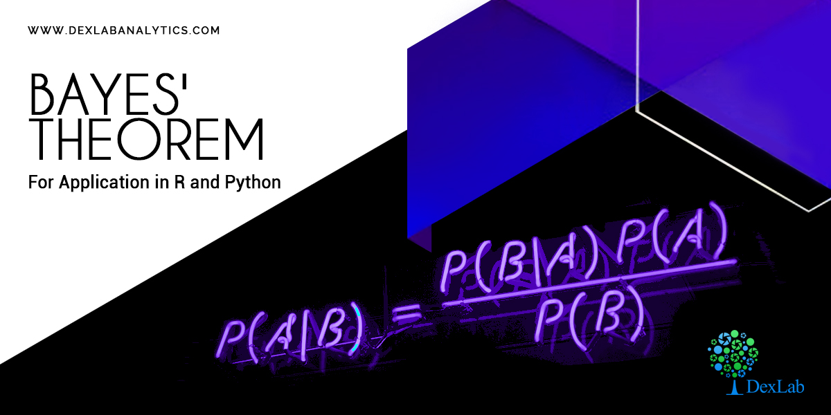
Bayes’ Theorem – Application in R and Python

Bayes’ Theorem – Application in R and Python

Bayes’ theorem, named after 18th century (1763) British mathematician Thomas Bayes, is a mathematical formula for determining conditional probability.  In the discussion of conditional probability we indicated that revising probability when new information is obtained is an important phase of probability analysis. Often, we begin our analysis with initial or prior probability estimates for specific events of interest. Then, from sources such as a sample, a special report, a product test, etc we obtain some additional information about the events. Given this new information, we update the prior probability values by calculating revised probabilities, referred to as posterior probabilities.

The steps involved in this probability revision process are depicted in the digram below:

  • Theorem:

An event A can occur only if one of the mutually exclusive and exhaustive set of events B1, B2,… ,Bn occurs. Suppose that the unconditional probabilities

And the conditional probabilities

are known. Then the conditional probability of a specified event Bi, when A is stated to have actually occurred, is given by

This is known as Bayes’ Theorem.

  • Proof:

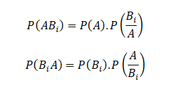
An event A can happen in mutually exclusive ways, B1 A, B2A,… Bn A, i.e. either when has occurred, or. So by the theorem of total probability


Again,

Since the events ABi and BiA are equivalent, their probabilities are also equal.

Hence

So that

Substituting for P(A) from above, the theorem is proved.

Equation (1) is also known as “Bayes” formula for calculating probabilities of hypothesis. Because B1, B2,…Bn may be considered as hypothesis which account for the occurrence of A. The probabilities P(B1),P(B2 ),…P(Bn) are called ‘a prior’ probabilities of the hypothesis.

While are known as a‘a posteriori’ probabilities of the same hypothesis.

Data Science Machine Learning Certification

For more on this, do peruse the Dexlab Analytics website today. Dexlab Analytics is a premiere institute for R programming courses in Gurgaon.


.
Machine Learning Jobs in 2019: Freezing your own Job

Machine Learning Jobs in 2019: Freezing your own Job

Machine Learning surely needs no introduction. Joining forces with Data Science and Big Data, Machine Learning is one of the principal technologies, which is carving the future for us. From self-propelled cars to voice assistants, to surgical robots, Artificial Intelligence is already amongst us.
Besides, with this cutting-edge technology, marketing is also witnessing a fresh bloom, irrespective of the field you are working on. Thus, it is obvious that the career opportunities have quickly and radically shifted in the way of the candidates who are well-versed with Machine Learning platforms and languages. If you are also looking forward to shooting your career up, the premium Machine Learning course in India is the place you should reach now!

2

Learning Machine Learning is No More a Pain Now!

Whether you are a professional or a fresher planning your way to be successful as a Machine Learning professional, you must ensure that you are updated. Besides, you should also be careful that you have certain skills in your grip that you can work on!

However, if you are not aware of them still, here are the skills that you need to focus on to rest assured:

Programming Languages

As you speak English and/or your regional languages accepted to your society in order to communicate comprehensibly, you also need to be well-versed with the languages specific to Machine Learning.

In a nutshell, R programming certification and Machine Learning Using Python are undoubtedly the most significant ones when it comes to Machine Learning.

Data Modeling

If you believe that you can already boast of considerable knowledge of R & Python, then you shall extend your knowledge a bit more towards the advanced methods of analysis. Brief know how of the coding structures, Data Modeling and Data Visualization will help you steer your career forwards.

Deep Learning and AI using Python

Statistics and Probability

If you are seeking to make a career out of Machine Learning, it is important to note that you should have a good grip of statistics and probability. Now, with the thorough courses of Python for Data Analysis along with extensive knowledge of statistics and probability from Dexlab Analytics, it will be easier than ever.

Besides all these, you also need to grasp significant insights into the improved algorithms and clustering methods. 


Interested in a career in Data Analyst?

To learn more about Data Analyst with Advanced excel course – Enrol Now.
To learn more about Data Analyst with R Course – Enrol Now.
To learn more about Big Data Course – Enrol Now.

To learn more about Machine Learning Using Python and Spark – Enrol Now.
To learn more about Data Analyst with SAS Course – Enrol Now.
To learn more about Data Analyst with Apache Spark Course – Enrol Now.
To learn more about Data Analyst with Market Risk Analytics and Modelling Course – Enrol Now.

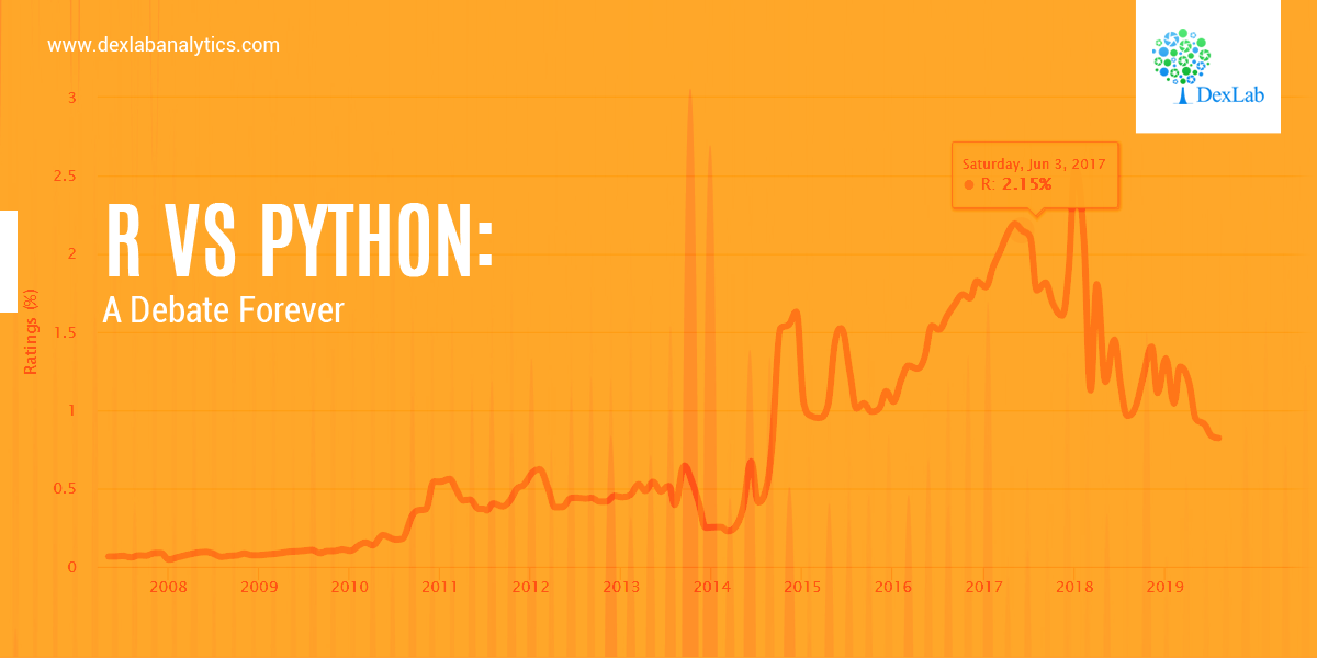
R Vs Python: A Debate Forever

R Vs Python: A Debate Forever

In this blog, we will bring forth the age old question and check which one is better, R programming and Python programming, when it comes to data science?

To be very honest, this question does not have a strict answer to it. However, in this blog we will lay down the key components of both the languages to give you a clearer picture. In the end, please decide for yourself and leave your comments in the section below.

The aim of this blog is to objectively put forward the pros and cons of both languages strictly from the perspective of data science.

We will discuss only about three main components, which are as follows:

  • Syntax
  • Performance
  • Applicability

There are other metrics, such as, trends in Industries and adaptation in the recent years which are beyond the scope of this blog. However, you can safely declare Python as the clear winner if those perspectives were concerned.

So let’s get started:

Syntax

Both R and Python are object-oriented languages. This is to say that everything is created as an object in which the information is mapped with the idea of using that object later in the analysis. However, when it comes to the syntax, i.e., the grammar of programming, R and Python are indeed very different.

R Programming

R programing is more suited to more seasoned coders who have prior experience of coding. The syntax is actually very similar to that of the previous languages, such as C, or C++ or Java and so on. The fundamental rules are that of C programming language. Also, use of semicolons is deemed optional in R. However, semicolons are necessary for multiple lines in a code inside a code block.

Deep Learning and AI using Python

Python

Python on the other hand, is the language more adaptable to the new generation of programmers. You can come from a non-programming background and still learn Python with relative ease.

Python is one of the most user friendly languages for the beginners. The syntax is designed to prioritize readability over preciseness of the code. In layman’s terms – coding in Python is very close to reading and writing with hand. In this regard, it is really popular amongst beginners in Data Science.

Performance

The performance is essentially measured by speed essentially when it comes to programming.

R Programming

As far as the general consensus goes R programming is much slower in terms of speed. The reason behind this is that R programming was initially designed to be used by statisticians for data analysis. Thus, R programming stresses more on precision than the speed.

Python

Python on the other hand, is relatively faster than R. Python offers the same level of precision whilst acting on a faster speed.

Note – The speed is taken into account independent of packages and libraries.

Applicability

Lastly, we will discuss the popular domains in which these languages are used.

2

R Programming

As mentioned above, R was developed specifically for statisticians. For this reason, R is mainly used in various research organizations and academia in general. However, R is now quickly being absorbed in the enterprises as well, mainly because of its popularity and the availability of a large number of packages for statistical computation.

Python

Python is a gene

As Python is a general-purpose programming language we can use to build different kinds of applications. We can use Python to build web applications using popular frameworks like Django or Flask.

Lately, Python is becoming popular amongst data scientists as the language of choice given the simplicity of syntax, high speed and performance it has to offer. There has been a trend which has seen a sharp rise in the adaptability of Python over R in the last few years in Data Science.

So, there you have it folks. Decide for yourself now! We will meet you soon in the next blog.

Dexlab Analytics is a pioneering institute of Data Science and Big Data Analytics with all-inclusive Big data courses in Delhi along with numerous other efficacious courses like Hadoop certification in Delhi, R programming courses in Gurgaon and Python for Data Analysis under experienced trainers and professionals.


Interested in a career in Data Analyst?

To learn more about Data Analyst with Advanced excel course – Enrol Now.
To learn more about Data Analyst with R Course – Enrol Now.
To learn more about Big Data Course – Enrol Now.

To learn more about Machine Learning Using Python and Spark – Enrol Now.
To learn more about Data Analyst with SAS Course – Enrol Now.
To learn more about Data Analyst with Apache Spark Course – Enrol Now.
To learn more about Data Analyst with Market Risk Analytics and Modelling Course – Enrol Now.

Statistical Application in R & Python: Normal Probability Distribution

Statistical Application in R & Python: Normal Probability Distribution

Gauss, the famous French Mathematician is responsible for developing one of the most significant distributions in all of statistics, i.e. – The Normal Distribution. Please refer to the blog on Central Limit Theorem: www.dexlabanalytics.com/blog/the-almighty-central-limit-theorem. It will help you fully grasp the significance of the Normal Distribution. However, if you want to revisit our series of blogs by following it from the start, you can reach STATISTICAL APPLICATION IN R & PYTHON: CHAPTER 1 – MEASURE OF CENTRAL TENDENCY right now!

Essentially, the Normal Distribution provides “approximations” to most other distributions such as the Binomial, Poisson, Gamma, Exponential, etc. This is to say as sample sizes get statistically large enough, most distributions approximate into a normal shaped curve.

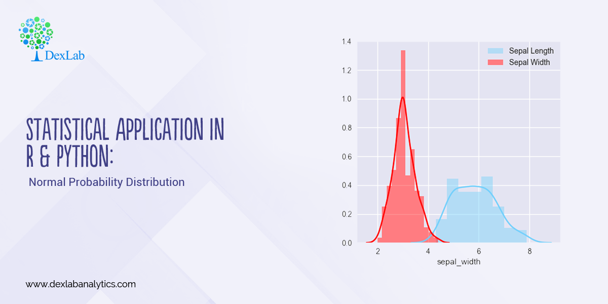
Every distribution has important features known as its “parameters”. Normal distribution has two parameters. These are Mean ( ) and Variance (σ²). The normal distribution has a bell-shaped curve, where the probability of likelihood peaks at its mean in the middle.

The Normal Distribution has vast practical applications in the field of Business, Finance, Medicine, and Physics and so on. Things like weights, heights, IQ scores follow the Normal Distribution.

Normal Distribution, Gaussian distribution, is a continuous probability distribution and is defined by the Probability Density Function (PDF).

Where,

Application:

Assume that the credit score fits a Normal Distribution.

Suppose Mr. Arjun’s last 10 month’s credit score are:

789, 635, 739, 687, 724, 810, 817, 735, 819, 820

What is the probability that the percentage of credit score will 825 or more in the 11th month?

Months

Credit Score

January

789

February

635

March

739

April

687

May

724

June

810

July

817

August

735

September

819

October

820


Calculating Normal Distribution in R:

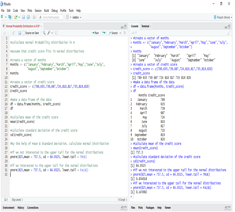
If we go to calculate Normal Probability Distribution in R, we can predict that the probability of the 11th month credit score will be 825 or greater than that is 14.60%, whereas in another case, the probability of the 11th month credit score will be 825 or less than that is 85.40%.

Calculate Normal Distribution in Python:

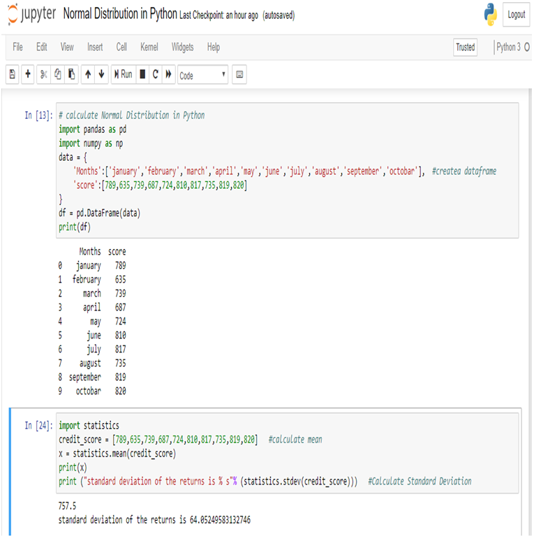
Make a data frame of the data and calculate Mean and Standard Deviation for calculate Normal Distribution.

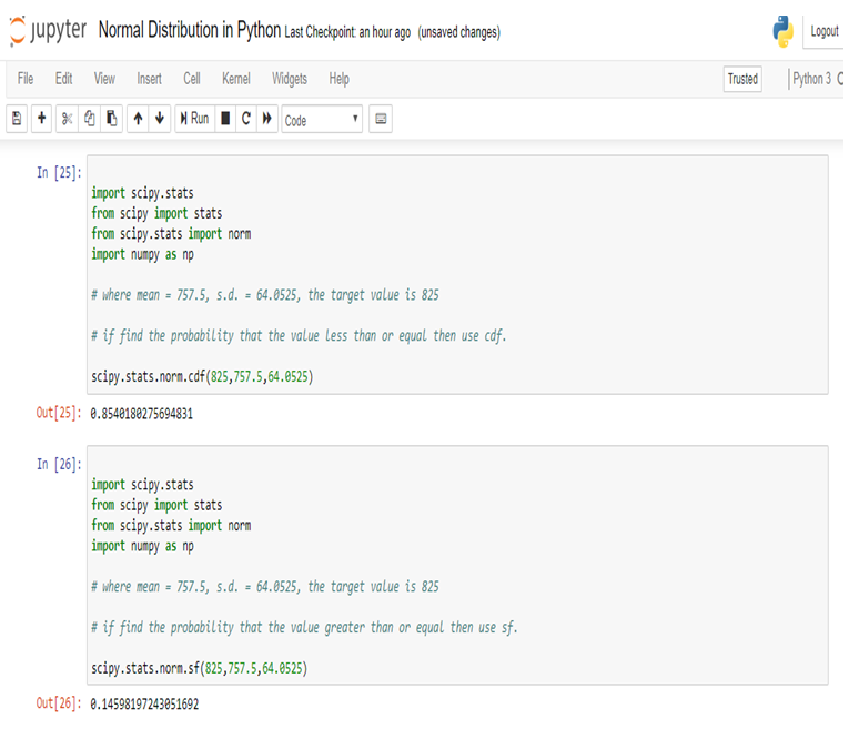
Now, we can easily calculate Normal Distribution in Python

So, in calculating the Normal Probability Distribution in Python, we can predict that the probability of the 11th month credit score will be 825 or greater than that is 14.60%, whereas in another case, the probability of the 11th month credit score will be 825 or less than that is 85.40%.

Conclusion:

Normal Distribution is used for calculating parameters. It is represented by the bell curve, where the total area of the curve is 1. Normal Distribution has its use in Finance, Business, Salaries, Blood Pressures, Measurement etc and many other fields.

Here, we have used Normal Distribution to predict Mr. Arjun’s 11th month credit score, and set the target (825). By Normal Distribution we can predict the percentage of possibility to achieve the target.

Calculating Binomial Distribution might be tricky for many but with Dexlab Analytics it won’t be hassle anymore. So, get hold of our STATISTICAL APPLICATION IN R AND PYTHON: CALCULATING BINOMIAL DISTRIBUTION blog, to get around all your problems.


Interested in a career in Data Analyst?

To learn more about Data Analyst with Advanced excel course – Enrol Now.
To learn more about Data Analyst with R Course – Enrol Now.
To learn more about Big Data Course – Enrol Now.

To learn more about Machine Learning Using Python and Spark – Enrol Now.
To learn more about Data Analyst with SAS Course – Enrol Now.
To learn more about Data Analyst with Apache Spark Course – Enrol Now.
To learn more about Data Analyst with Market Risk Analytics and Modelling Course – Enrol Now.

Statistical Application in R and Python: Calculating Binomial Distribution

Statistical Application in R and Python: Calculating Binomial Distribution

In this blog, we will take a look at the Binomial distribution. This blog is among the series of blogs through which you’ll have a vivid idea of the Statistical Application using R and Python. Statistical Application In R & Python: Chapter 1 – Measure Of Central Tendency is the first of such blogs.

The binomial distribution is an extension of the Bernoulli distribution. In Bernoulli, we have only one parameter, i.e. the probability of success.

Now, consider a case where we have “n” number of trials and we want to predict the probability of success from it. This is the Binomial case.

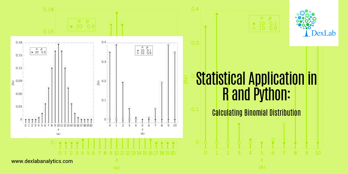
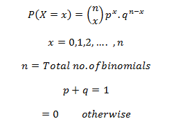
Binomial distribution has two parameters, i.e.: number of trails (n) AND probability of success (p). The mean of the binomial is a product of its two parameters, i.e. n multiplied by p. It is a discrete probability distribution. Here, each trial is assumed to have only two outcomes, either success or failure.

If X be a discrete random variable (taking only non-negative values), it is said to be following binomial distributions with a probability mass function as:-


Application:

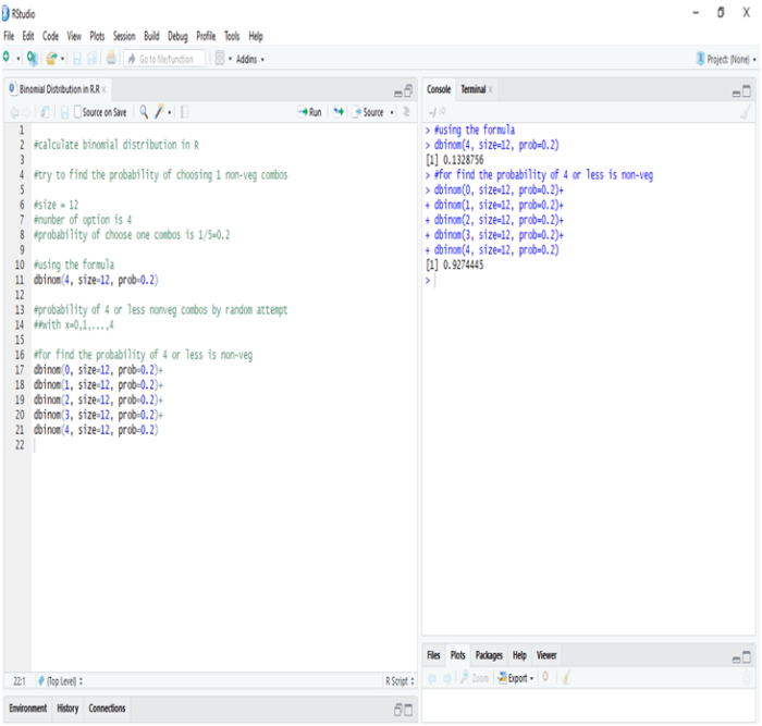
A food shop starts a offer for a festive season, They have 12 different baskets, each basket has 5 combos and only 1 of them is non-veg. Find the probability of having 4 or less non-veg combos, if a consumer tries every combos at random.

Since, only 1 out of 5 combos is non-veg, the probability of choose a non-veg combos by random is 1/5 = 0.2

Calculate Binomial Distribution in R:

In R the probability of one non-veg combos choose by random in 5 is 13.28%, whereas the probability of four or less combos choose by random in a twelve baskets is 92.44%

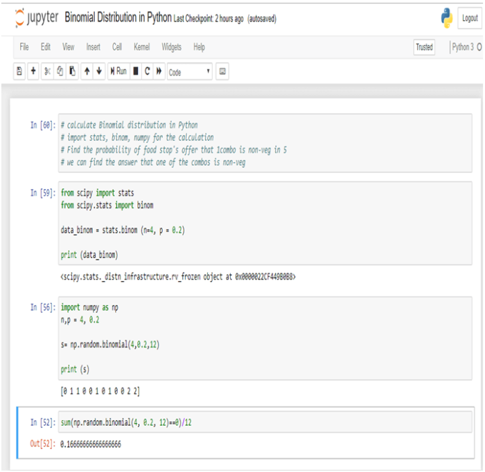
Calculate Binomial Distribution in Python:

In Python the probability of one non-veg combos choose by random in 5 is 16.66%.

Conclusion:-

Binomial Distribution is the process by which we can calculate the probability of success from “n” number of trails. In Binomial Distribution we can find only two outcomes like “Yes” or “No”.

Dexlab Analytics is a pioneering institute of Data Science, with peerless trainers to help you ease your journey with Python Certification, R Programming Certification and Big Data Certification along with numerous other advanced and/or career oriented courses in Computer Science.


Interested in a career in Data Analyst?

To learn more about Data Analyst with Advanced excel course – Enrol Now.
To learn more about Data Analyst with R Course – Enrol Now.
To learn more about Big Data Course – Enrol Now.

To learn more about Machine Learning Using Python and Spark – Enrol Now.
To learn more about Data Analyst with SAS Course – Enrol Now.
To learn more about Data Analyst with Apache Spark Course – Enrol Now.
To learn more about Data Analyst with Market Risk Analytics and Modelling Course – Enrol Now.

Calculating the Standard Deviation Using R & Python

Calculating the Standard Deviation Using R & Python

When it comes to summarizing the data, standard deviation (σ) is the value which tells us about the spread of the data. More specifically, it gives information about the dispersion of each observation from the mean of the data. Now, if you are interested in understanding Mean and knowing how to calculate it, then we have shown you in CALCULATING GEOMETRIC MEAN USING R AND PYTHON And APPLICATION OF HARMONIC MEAN USING R AND PYTHON.

Thus, in essence standard deviation gives us valuable information about the robustness of the mean. The deviation is in both positive and negative direction of the mean.

Therefore, it is desirable for the standard deviation to be a low value in comparison to the mean. This would indicate a smaller spread.

Mathematically speaking, standard deviation is known as the second moment about Mean. Variance is standard deviation squared. The variance does not have any mathematical significance on its own. Think of the variance as a mere mathematical maneuver.

The formula for the Variance is:

Application:

An investor wants to calculate the Standard Deviation experience by his investment portfolio in last 12 months (Year 2017-2018).  The returns are:-

Month (Year 2017-18)

Returns (%)

April

12%

May

10%

June

-8%

July

4%

August

12.25%

September

18%

October

13%

November

-9%

December

-4%

January

3%

February

9%

March

11.05%

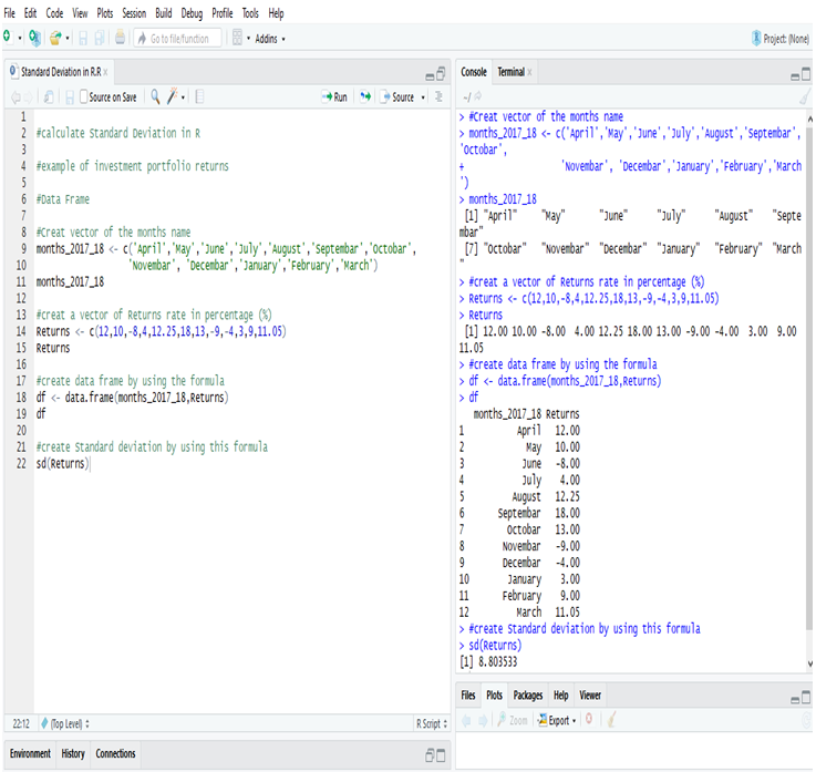
Calculate Standard Deviation in R:

Examining the Standard Deviation of the investment portfolio returns of a year in R, we get the deviation = 8.803533 or, 8.81% (Approx).

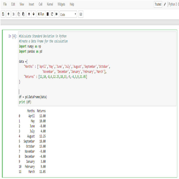
Calculate Standard Deviation in Python:

First, create a Data Frame in Python.

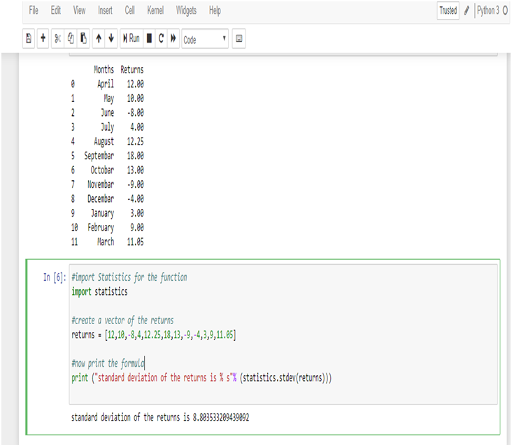
Now, calculate Standard Deviation of the returns,

Examining the Standard Deviation of the investment portfolio returns of a year in Python, we get the deviation = 8.803533209439092 or, 8.81% (Approx)

Standard Deviation is a key part of calculating margins of errors.

Standard deviation shows the variation from the mean. A low standard deviation indicates that the observations (series of number) are very close to the mean. A high standard deviation indicates that the observations (series of numbers) are spread out over a large range.

In this data the mean of the returns is 5.95%, and standard deviation is 8.81% which is close to the mean. So, the deviation of the data is low.

Thus, the investor now knows that the returns of his portfolio fluctuate by approximately 8.81% month-over-month. The information can be used to modify the portfolio to better the investor’s attitude towards risk. If the investor is risk-loving and is comfortable with investing in higher-risk, higher-return securities and can tolerate a higher standard deviation, he/she may consider adding in some small-cap stocks or high-yield bonds. Conversely, an investor who is more risk-averse may not be comfortable with this standard deviation and would want to add in safer investments such as large-cap stocks or mutual funds.

Endnotes

This article will surely help you to figure out the standard deviation with R and Python. However, if you want to have a general idea about Central tendency, about Mean, Median and Mode, then go through our blog on STATISTICAL APPLICATION IN R & PYTHON: CHAPTER 1 – MEASURE OF CENTRAL TENDENCY.

For all other information about us and our courses, Dexlab Analytics is there with you. You can also follow us on Facebook and LinkedIn and go through our blogs to stay updated always.


Interested in a career in Data Analyst?

To learn more about Data Analyst with Advanced excel course – Enrol Now.
To learn more about Data Analyst with R Course – Enrol Now.
To learn more about Big Data Course – Enrol Now.

To learn more about Machine Learning Using Python and Spark – Enrol Now.
To learn more about Data Analyst with SAS Course – Enrol Now.
To learn more about Data Analyst with Apache Spark Course – Enrol Now.
To learn more about Data Analyst with Market Risk Analytics and Modelling Course – Enrol Now.

Application of Median Using R And Python: Calculating Median On the Go

Application of Median Using R And Python: Calculating Median On the Go

This blog is in continuation of STATISTICAL APPLICATION IN R & PYTHON: CHAPTER 1 – MEASURE OF CENTRAL TENDENCY and takes you through a comprehensive way to calculate the Median in R and Python.

The term ‘Median’ is derived from the Latin word – ‘Medius’ means the center of something. In mathematics, Median is treated is that unique observation which would divide your data set into two equal halves.

If you are still unclear about Mean and/or seeking easier ways to calculate Mean using R & Python, then check APPLICATION OF HARMONIC MEAN USING R AND PYTHON and CALCULATING GEOMETRIC MEAN USING R AND PYTHON.

Median is special because unlike its rival, the Mean, Median is not ridiculed by the curse of extreme values. To illustrate the curse of extreme values, we bring you the following example:

Imagine I had the following data about the average annual salaries:

In Lacs

8.5
9
11
7
8
8.5
36

The mean of the above data set is: 88/7 = 12.57 lacs.

Whereas, to get the median we would have to first arrange the data into ascending order and look for the midpoint of my data i.e.,(1/2 + n/2)th observation. Where “n” is the number of observations.

The median would then be:

7
8
8.5
8.5
9
11
36

Median is the 4th observation, which is 8.5 lacs.

Looking at the mean and median, it would be fair to conclude that median is the better choice to accurate summarizing the data set whenever extreme values are present. However, this may be a crude generalization which should be taken with a pinch of salt. Despite its flaws, the mean still has statistical properties used in predictive analytics which the median lacks.

Application:

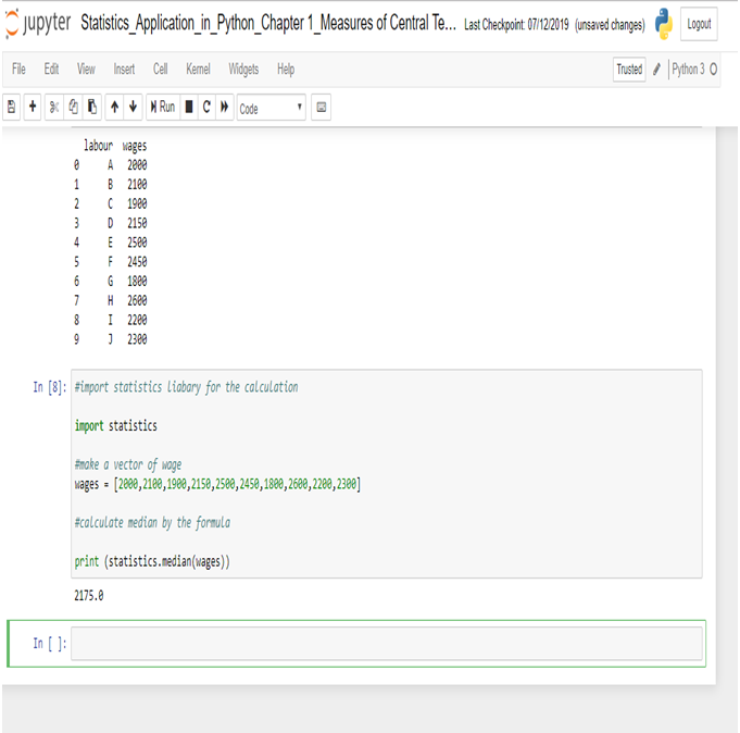
A construction company gave wages to their 10 labor (Let name A to J)  as a weekly basis, the wages are 2000, 2100, 1900, 2150, 2500, 2450, 1800, 2600, 2200, 2300. Compute the Median wages of the construction company.

Sr.NoLaborsWages (Weekly)
1A2000
2B2100
3C1900
4D2150
5E2500
6F2450
7G1800
8H2600
9I2200
10J2300

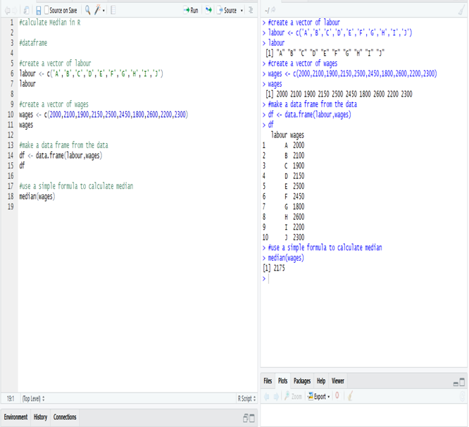
Calculation Median in R:

Python Certification

The Median wage is 2175, calculate in R.

Calculate Median in Python:

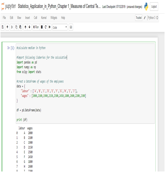
Create a data frame of the data in Python.

R Programming Certification

Now, calculate Median in Python.

R Programming Certification

The Median wage is 2175, calculated in R.

This concludes the post. If you have any queries with regards to this post, you can reach us at Dexlab Analytics. Furthermore, you can also look up for interesting and quality courses of R Programming Certification, Python Certification. Also, you can enroll with us for our combined courses of Data Science with Python Certification, Deep Learning and AI using Python, among others. So, hurry up and grab the best course!


Interested in a career in Data Analyst?

To learn more about Data Analyst with Advanced excel course – Enrol Now.
To learn more about Data Analyst with R Course – Enrol Now.
To learn more about Big Data Course – Enrol Now.

To learn more about Machine Learning Using Python and Spark – Enrol Now.
To learn more about Data Analyst with SAS Course – Enrol Now.
To learn more about Data Analyst with Apache Spark Course – Enrol Now.
To learn more about Data Analyst with Market Risk Analytics and Modelling Course – Enrol Now.

Calculating Geometric Mean Using R and Python

Calculating Geometric Mean Using R and Python

In this blog, we are going to discuss the Geometric Mean and its application using Python and R.

Geometric Mean of group of ‘n’ observations is the nth root of their product. It is defined only when all observations have the same sign and none of them is zero.

Application:

Calculate the Geometric Mean of the salary increment of 12 employees. From the following table, calculate the average salary increment of the year (2019-2020):-


Name

Salary Increment in

Percentage (%)

Ritesh

10.09%

Heena

15.45%

Kritika

9%

Anuradha

13.06%

Gaurav

20%

Prakash

14%

Aarti

16%

Meena

6.25%

Utkarsh

12.85%

Chirag

10%

Neha

18%

Smrita

21.36%


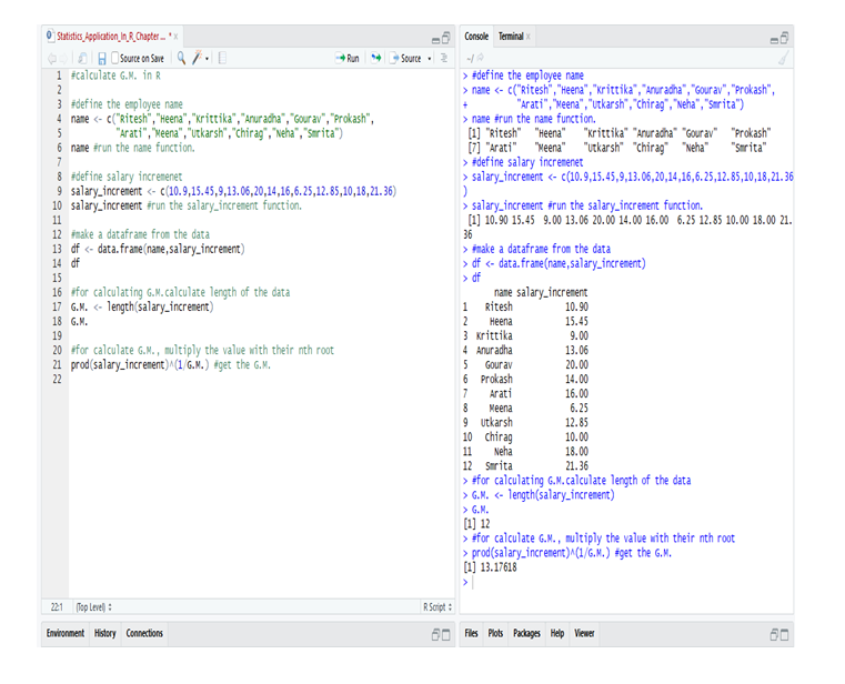
Calculate the Geometric Mean in R:

So, from the data of the employee’s in R we calculate the G.M. and get that the average salary increment in the year (2019-2020) = 13.17618 or 13.18% (approx).

Calculate the Geometric Mean in Python:

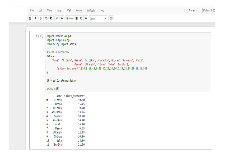
First, make a data frame in Python from the following table.

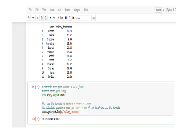
Now, calculate the Geometric Mean from the data-frame.

So, from the data of the employee’s in Python we calculate the G.M. and get that the average salary increment in the year (2019-2020) = 13.176183416401196 or 13.18% (approx).

We use Geometric Mean for calculating ratios, rates and percentages. And it is not affected by the extreme value or outlier. In this particular problem, we use Geometric Mean because an average of the salary increment of the employee’s not affected by the extreme highest or extreme lowest value, that’s why the salary increment rates of Meena and Smrita do not have any effect on the total average rate.

Geometric Mean gives small value than Arithmetic Mean.

2

Note: This is a continuation of the blog: Statistical Application in R & Python: Chapter 1 – Measure of Central Tendency. It would be better to go through the first installment and then read this one. More blogs are to be followed, so stay tuned.

DexLab Analytics is a premier Python training institute in Delhi. Our industry-relevant courses are carefully crafted by experts. Follow us on Facebook and Instagram.


Interested in a career in Data Analyst?

To learn more about Data Analyst with Advanced excel course – Enrol Now.
To learn more about Data Analyst with R Course – Enrol Now.
To learn more about Big Data Course – Enrol Now.

To learn more about Machine Learning Using Python and Spark – Enrol Now.
To learn more about Data Analyst with SAS Course – Enrol Now.
To learn more about Data Analyst with Apache Spark Course – Enrol Now.
To learn more about Data Analyst with Market Risk Analytics and Modelling Course – Enrol Now.

Call us to know more