Python Programming training Archives - DexLab Analytics | Big Data Hadoop SAS R Analytics Predictive Modeling & Excel VBA

ARIMA (Auto-Regressive Integrated Moving Average)

Posted on January 27, 2021February 13, 2021 by Dexlab

This is another blog added to the series of time series forecasting. In this particular blog I will be discussing about the basic concepts of ARIMA model.

So what is ARIMA?

ARIMA also known as Autoregressive Integrated Moving Average is a time series forecasting model that helps us predict the future values on the basis of the past values. This model predicts the future values on the basis of the data’s own lags and its lagged errors.

When a data does not reflect any seasonal changes and plus it does not have a pattern of random white noise or residual then an ARIMA model can be used for forecasting.

There are three parameters attributed to an ARIMA model p, q and d :-

p :- corresponds to the autoregressive part

q:- corresponds to the moving average part.

d:- corresponds to number of differencing required to make the data stationary.

In our previous blog we have already discussed in detail what is p and q but what we haven’t discussed is what is d and what is the meaning of differencing (a term missing in ARMA model).

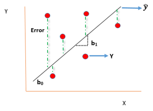
Since AR is a linear regression model and works best when the independent variables are not correlated, differencing can be used to make the model stationary which is subtracting the previous value from the current value so that the prediction of any further values can be stabilized . In case the model is already stationary the value of d=0. Therefore “differencing is the minimum number of deductions required to make the model stationary”. The order of d depends on exactly when your model becomes stationary i.e. in case the autocorrelation is positive over 10 lags then we can do further differencing otherwise in case autocorrelation is very negative at the first lag then we have an over-differenced series.

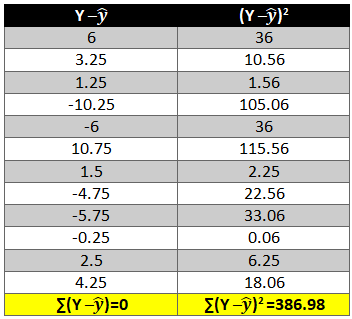
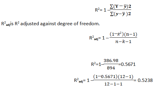
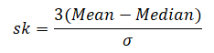
The formula for the ARIMA model would be:-

To check if ARIMA model is suited for our dataset i.e. to check the stationary of the data we will apply Dickey Fuller test and depending on the results we will using differencing.

In my next blog I will be discussing about how to perform time series forecasting using ARIMA model manually and what is Dickey Fuller test and how to apply that, so just keep on following us for more.

So, with that we come to the end of the discussion on the ARIMA Model. Hopefully it helped you understand the topic, for more information you can also watch the video tutorial attached down this blog. The blog is designed and prepared by Niharika Rai, Analytics Consultant, DexLab Analytics DexLab Analytics offers machine learning courses in Gurgaon. To keep on learning more, follow DexLab Analytics blog.

Theory of Estimation Part-I: The Introduction

Posted on November 27, 2020November 27, 2020 by Dexlab

The theory of estimation is a branch in statistics that provides numerical values of the unknown parameters of the population on the basis of the measured empirical data that has a random component. This is a process of guessing the underlying properties of the population by observing the sample that has been taken from the population. The idea behind this is to calculate and find out the approximate values of the population parameter on the basis of a sample statistics.

Population:- All the items in any field of inquiry constitutes to a “Population”. For example all the employees of a factory is a population of that factory and the population mean is represented and the size of the population is represented by N.

Sample:- Selection of few items from the population constitutes to a sample and the mean of the sample is represented by and the sample size is represented by n

Statistics:- Any statistical measure calculated on the basis of sample observations is called Statistic. Like sample mean, sample standard deviation, etc.

Estimator:- In general estimator acts as a rule, a measure computed on the basis of the sample which tells us how to calculate the values of the estimate. It is a functional form of all sample observations prorating a representative value of the collected sample.

Suppose we have a random sample x_1,x_2,…,x_n on a variable x, whose distribution in the population involves an unknown parameter. It is required to find an estimate of on the basis of sample values.

Unbiasedness:-A statistic t is said to be an unbiased estimator if E(β ̂)= βi.e. observed value is equal to the expected value. In case E(β ̂)≠ β then the estimator is biased estimator.

Consistency:- One of the most desirable property of good estimator is that its accuracy should increase when the sample becomes larger i.e. the error between the expected value and the observed value reduces as the size of the sample increases E(β ̂ )- β=0

Efficiency:-An estimator is said to be an efficient estimator if it has the smallest variance compared to all the consistent and unbiased estimators. If consistent estimator exists whose sampling variance is less than that of any other consistent estimator, it is said to be “most efficient”; and it provides a standard for the measurement of ‘efficiency’ of a statistic.

Sufficiency:- An estimator is said to be sufficient if it contains all information in the sample about .

At the end of this discussion, hopefully, you have learned what theory of estimation is. Watch the video tutorial attached below to learn more about this. DexLab Analytics is a data science training institute in gurgaon, that offers advanced courses. Follow the blog section to access more informative posts like this.

An Introductory Guide to NumPy

Posted on November 25, 2020November 25, 2020 by Dexlab

NumPy also known as numerical python, is a library consisting of multidimensional array objects and a collection of routines for processing those arrays. Using NumPy, mathematical and logical operations on arrays can be performed without it which was not possible. For example-

Multiplication of two lists will cause an error as a data structure like lists, tuple, dictionaries and sets do not allow mathematical operations.

Therefore we need NumPy to covert our data structures like lists into 1d, 2d, 3d or nd arrays so that mathematical operations can be performed. U

We can use .array() methods to create these arrays.

Now let’s check out few examples and also perform few mathematical operations to have a better understanding.

In the above code we first import NumPy library and then use .array() method to two 1d-array a1 and b1 using the list we previously created.
Now let’s multiply a1 and b1 array.
Now let’s use .array() method to directly create an array.

Arrays can be created using lists, tuples and dictionaries as you can see in the above example.

Now for 2-d arrays recall that we can also make list of lists. Let’s use that to create 2d-arrays.

2d-arrays can also be created using tuples.

Remember that we are not using these as matrices because matrix multiplication is an entirely different thing we are just trying to perform mathematical operations which were otherwise not possible.

Random Module

Numpy also has various ways with which we can create array of random numbers which then can be used in number of ways like generating a data for practice purposes or for building beautiful graphs for a presentation.

Given below is a list of type of random numbers you can generate

.rand() :- This particular method helps you generate uniformly distributed random numbers i.e. numbers between 0 and 1 where each number between 0 and 1 will have equal probability to be in the sample dataset.

The above code generates a 2d-array with values between 0 and 1.

.randn():- This method generates normally distributed random numbers i.e. numbers between -3 and +3 where mean=median=mode and ploted gives a bell shaped curve.

Here the 20 random numbers are generated ranging between -3 and + 3.

Note:- Remember that the data is randomly picked from the normally distributed values between -3 and +3 so the graph is not bell shaped but the original data from which the values are being picked randomly is bell shaped with mean=median-mode.

.randint():-This method generates random integers between a given range.

So, with that we come to the end of the discussion on the Numpy. Hopefully it helped you understand Numpy, for more information you can also watch the video tutorial attached down this blog. DexLab Analytics offers machine learning courses in delhi. To keep on learning more, follow DexLab Analytics blog.

Linear Regression Part II: Predictive Data Analysis Using Linear Regression

Posted on November 23, 2020November 23, 2020 by Dexlab

In our previous blog we studied about the basic concepts of Linear Regression and its assumptions and let’s practically try to understand how it works.

Given below is a dataset for which we will try to generate a linear function i.e.

y=b₀+b₁Xi

Where,

y= Dependent variable

Xi= Independent variable

b₀ = Intercept (coefficient)

b₁= Slope (coefficient)

To find out beta (b₀& b₁) coefficients we use the following formula:-

Let’s start the calculation stepwise.

First let’s find the mean of x and y and then find out the difference between the mean values and the X_i and Y_ie. (x-x ̅ ) and (y-y ̅ ).
Now calculate the value of (x-x ̅ )² and (y-y ̅ )². The variation is squared to remove the negative signs otherwise the summation of the column will be 0.
Next we need to see how income and consumption simultaneously variate i.e. (x-x ̅ )* (y-y ̅ )

Now all there is left is to use the above calculated values in the formula:-

As we have the value of beta coefficients we will be able to find the y ̂(dependent variable) value.

We need to now find the difference between the predicted y ̂ and observed y which is also called the error term or the error.

To remove the negative sign lets square the residual.

What is R²and adjusted R² ?

R² also known as goodness of fit is the ratio of the difference between observed y and predicted and the observed y and the mean value of y.

Hopefully, now you have understood how to solve a Linear Regression problem and would apply what you have learned in this blog. You can also follow the video tutorial attached down the blog. You can expect more such informative posts if you keep on following the DexLab Analytics blog. DexLab Analytics provides data Science certification courses in gurgaon.

Linear Regression Part I: A Comprehensive Guide to Linear Regression

Posted on November 9, 2020November 9, 2020 by Dexlab

Today’s blog explores another vital statistical concept Linear Regression, let’s begin. Linear regression is normally used in statistics for predictive modeling. It tries to model a relationship between two independent (explanatory variable) and dependent (explained variable) variables X and Y by fitting a linear equation (Y=b_o+b₁X+U_i) to an observed data.

Assumptions of linear regression

U_i is a random real variable, where U_iis the difference between the observed dependent variable Y and predicted Y variable.
The mean of U_iin any particular period is zero.
The variance of U_i is constant in each period i.e for all values of X, U_i will show the same dispersion around their mean
The variable U_i has a normal distribution i.e the value of U_i (for each X_i) have a bell shaped symmetrical distribution about their zero mean.
The random terms of different observations are independent i.e the covariance of any U_iwith any other U_j is equal to zero.
U_i is independent of the explanatory variable X.
X_iare a set of fixed values in the hypothesised process of repeated sampling which underlies the linear regression model.
In case there are more than one explanatory variables then they are not perfectly linearly correlated.

Linear Regression equation can be written as:

Where,

is the dependent variable

X is the independent variable.

b₀is the intercept (where the line crosses the vertical y-axis)

b₁is the slope

U_i is the error term (difference between ) also called residual or white noise.

Simple linear regression follows the properties of Ordinary Least Square (OLS) which are as follows:-

Unbiased estimator:- E()=b ie. an estimator is unbiased if its bias is 0; E() – b = 0
Minimum Variance:- An estimate is best when it has the smallest variance as compared to any other estimate obtained from other econometric method.
Efficient estimator:- When it has both the previous properties ie.
Linear estimator
Best, Linear, Unbiased estimator (BLUE)
Minimum mean squared error (MSE) estimator:- It is a combination of the unbiasedness and minimum variance properties. An estimator is a minimum MSE estimator if it has the smallest mean square error.

With that the discussion on Linear Regression wraps up here, hopefully it cleared away any confusion you might have and helped you get a grasp on the concept. We have a video discussion on this same topic, which is attached below this blog, check it out for further reference.

Continue to track the DexLab Analytics blog to find informative posts related to Python for data science training.

Why Pursuing a Certification Course in Machine Learning Makes Sense Than Doing Self-Study?

Posted on November 6, 2020November 6, 2020 by Dexlab

If you are aware of the growth opportunities awaiting you in the Machine Learning domain, you must be in a rush to master the Machine Learning skills. Now, there are courses available that aim to sharpen the students with skills they would need to work in a challenging environment. However, some often prefer the self-study mode for developing knowledge in this highly specialized domain. No matter which way you prefer to learn, ultimately your passion and dedication would matter the most, because in both ways you need to put in the hard work and really toil hard to make any progress.

Is self-study a feasible option?

If you have already been through some course and want to go to the advanced level through self-study that’s a different issue, but, for those who are just starting out without any background in science, does it even make any sense to opt for self-study?

Given the way Machine Learning technology is moving fast and creating a demand for professionals with highly specialized industry knowledge, do you think self-study would be enough? Do you think a self-study plan to learn something you have no idea about would work? How much time would you need to devote? What should be your learning route? And how do you know this is the right path to follow?

Before we dive deeper into the discussion, we need to go through some prerequisites for Machine Learning study plan.

Machine learning is a broad field and assuming you are a beginner with no prior knowledge in this domain, you have to be familiar with mathematics, statistics, programming languages, meaning undergoing a Python certification training</strong>, must be proficient in data handling including analysis and modeling, you have to work on algorithms. So, can you pick up all of these skills one by one via self-study? Add to the list the latest Machine Learning tools and applications you need to grasp.

There will be help available in the form of:

There would be vast resources, in forms of e-books, lectures, video tutorials, most of these are free and easily accessible.

There are forums, groups out there which you can join and access help

You can take part in online competitions

Think it through. How long will it take for you to get from one stage to the next?

Even though there being no dearth of resources available you would be struggling with your progress and most importantly you would struggle to keep up with the pace the technology is moving ahead. Picking up a programming language, grasping and mastering concepts of linear algebra, probability, data is going to be a mammoth task.

What difference a certification course can make?

To begin with these courses are designed for people coming from different backgrounds, so, you having or, not having any prior knowledge in mathematics, statistics wouldn’t matter as you would be taught everything from scratch be it math or, Machine Learning Using Python.

The programs are designed for both working professionals as well as for beginners, all you need to do is choose the one that suits your specific level.

These courses are designed to transform you into an industry-ready professional and you would be under the guidance of professionals who are more than familiar with the nuances of the way the industry functions.

The modules would follow a strict schedule and your training path would be well planned out covering all the areas you need to master.

You would learn via hands-on training and get to handle projects. Nothing makes you skilled like hands-on training.

Your journey towards a smarter future needs to be through a well mapped-out path, so, be smart about it. DexLab Analytics offers industry-ready courses on Data Science, Machine Learning course in Gurgaon and AI with Python. Take advantage of the courses that are taught by instructors who have both expertise and experience. Time is indeed money, so, stop wasting time and get down to learning.

Introducing Automation: Learn to Automate Data Preparation with Python Libraries

Posted on October 27, 2020December 12, 2020 by Dexlab

In this blog we are discussing automation, a function for automating data preparation using a mix of Python libraries. So let’s start.

Problem statement

A data containing the following observation is given to you in which the first row contains column headers and all the other rows contains the data. Some of the rows are faulty, a row is faulty if it contains at least one cell with a NULL value. You are supposed to delete all the faulty rows containing NULL value written in it.

In the table given below, the second row is faulty, it contains a NULL value in salary column. The first row is never faulty as it contains the column headers. In the data provided to you every cell in a column may contain a single word and each word may contain digits between 0 & 9 or lowercase and upper case English letters. For example:

In the above example after removing the faulty row the table looks like this:

The order of rows cannot be changed but the number of rows and columns may differ in different test case.

The data after preparation must be saved in a CSV format. Every two successive cells in each row are separated by a single comma ‘,’symbol and every two successive rows are separated by a new-line ‘\n’ symbol. For example, the first table from the task statement to be saved in a CSV format is a single string ‘S. No., Name, Salary\n1,Niharika,50000\n2,Vivek,NULL\n3,Niraj,55000’ . The only assumption in this task is that each row may contain same number of cells.

Write a python function that converts the above string into the given format.

Write a function:

def Solution(s)

Given a string S of length N, returns the table without the Faulty rows in a CSV format.

Given S=‘S. No., Name, Salary\n1,Niharika,50000\n2,Vivek,NULL\n3,Niraj,55000’

The table with data from string S looks as follows:

After removing the rows containing the NULL values the table should look like this:

You can try a number of strings to cross-validate the function you have created.

Let’s begin.

First we will store the string in a variable s

Now we will start by declaring the function name and importing all the necessary libraries.

Creating a pattern to separate the string from ‘\n’ .

Creating a loop to create multiple lists within a list.

In the above code the list is converted to an array and then used to create a dataframe and stored as csv file in the default working directory.

Now we need to split the string to create multiple columns.

The above code creates a dataframe with multiple columns.

Now after dropping the rows with NaN values data looks like

To reset the index we can now use .reset_index() method.

Now the problem with the above dataframe created is that the NULL values are in string format, so first we need to convert them into NaN values and then only we will be able to drop them. For that we will be using the following code.

Now we will be able to drop the NaN values easily by using .dropna() method.

In the above code we first dropped the NaN values then we used the first row of the data set to create column names and then dropped the original row. We also made the first column as index.

Hence we have managed to create a function that can give us the above data. Once created this function can be used to convert a string into dataframe with similar pattern.

Hopefully, you found the discussion informative enough. For further clarification watch the video attached below the blog. To access more informative blogs on Data science using python training related topics, keep on following the Dexlab Analytics blog.

Here’s a video introduction to Automation. You can check it down below to develop a considerable understanding of the same:

How IoT analytics can help your business grow?

Posted on October 6, 2020October 6, 2020 by Dexlab

Internet of Things or IOT devices are a rage now, as these devices staying connected to the internet can procure data and exchange the same using the sensors embedded in those. Now the data which is being generated in copious amount needs to be processed and in comes IoT Analytics. This platform basically is concerned with analyzing the large amount of data generated by the devices. The interconnectivity of devices is helping different sectors be in sync with the world, and the timely extraction of data is of utmost significance now as it delivers actionable insights. This is a highly skilled job responsibility that could only be handled by professionals having done artificial intelligence course in delhi.

This particular domain is in the nascent stage and it is still growing, however, it is needless to point out that IoT analytics holds the clue to business success, as it enables the organizations to not only extract information from heterogeneous data but also helps in data integration. With the IoT devices generating almost 5 quintillion bytes of data, it is high time the organizations start investing in developing IoT analytics platform and building a data expert team comprising individuals having a background in Machine Learning Using Python. Now let’s have a look at the ways IoT analytics can boost business growth.

Optimized automated work environment

IoT analytics can optimize the automated work environment, especially the manufacturing companies can keep track of procedures without involving human employees and thereby lessening the chances of error and enhancing the accuracy of predicting machine failure, with the sensors monitoring the equipments and tracing every single issue in real-time and sending alerts to make way for predictive maintenance. The production flow goes on smoothly as a result without developing any glitch.

Increasing productivity

In an organization gauging the activity of the employees assumes huge significance as it directly impacts the productivity of the company, with sensors being strategically placed to monitor employee activity, performance, moods and other data points, this job gets easier. The data later gets analyzed to give the management valuable clues that enable them to make necessary modifications in policies.

Bettering customer experience

Regardless of the nature of your business, you would want to make sure that your customers derive utmost satisfaction. With IoT data analytics in place you are able to trace their preferences thanks to the data streaming from devices where they have already left a digital footprint of their shopping as well as searching patterns. This in turn enables you to offer tailor-made service or products. Monitoring of customer behavior could lead to devising marketing strategies that are information based.

Staying ahead by predicting trends

One of the crucial aspects of IoT analytics is its ability to predict future trends. As the smart sensors keep tracking data regarding customer behavior, product performance, it becomes easier for businesses to analyze future demands and also the way trends will change to make way for emerging ones and it enables the businesses to be ready. Having access to a future estimate prepares not just businesses but industries be future ready.

Smarter resource management

Efficient utilization of resources is crucial to any business, and IoT analytics can help in a big way by making predictions on the basis of real-time data. It allows companies to measure their current resource allocation plan and make adjustments to make optimal usage of the available resources and channelizing that in the right direction. It also aids in disaster planning.

Ever since we went digital the streaming of large quantity of data has become a reality and this is going to continue in the coming decades. Since, most of the data generated this way is unstructured there needs to be cutting edge platforms like IoT analytics available to manage the data and processing it to enable industries make informed decisions. Accessing Data Science training, would help individuals planning on making a career in this field.

Skewness and Kurtosis: A Definitive Guide

Posted on September 29, 2020September 29, 2020 by Dexlab

While dealing with data distribution, Skewness and Kurtosis are the two vital concepts that you need to be aware of. Today, we will be discussing both the concepts to help your gain new perspective.

Skewness gives an idea about the shape of the distribution of your data. It helps you identify the side towards which your data is inclined. In such a case, the plot of the distribution is stretched to one side than to the other. This means in case of skewness we can say that the mean, median and mode of your dataset are not equal and does not follow the assumptions of a normally distributed curve.

Positive skewness:- When the curve is stretched towards the right side more it is called a positively skewed curve. In this case mean is greater than median and median is the greater mode

(Mean>Median>Mode)

Let’s see how we can plot a positively skewed graph using python programming language.

First we will have to import all the necessary libraries.

Then let’s create a data using the following code:-

In the above code we first created an empty list and then created a loop where we are generating a data of 100 observations. The initial value is raised by 0.1 and then each observation is raised by the loop count.

To get a visual representation of the above data we will be using the Seaborn library and to add more attributes to our graph we will use the Matplotlib methods.

In the above graph you can see that the data is stretched towards right, hence the data is positively skewed.

Now let’s cross validate the notion that whether Mean>Median>Mode or not.

Since each observation in the dataset is unique mode cannot be calculated.

Calculation of skewness:

Formula:-

In case we have the value of mode then skewness can be measured by Mode ─ Mean

In case mode is ill-defined then skewness can be measured by 3(Mean ─ Median)

To obtain relative measures of skewness, as in dispersion we use the following formula:-

When mode is defined:-
When mode is ill-defined:-

To calculate positive skewness using Python programming language we use the following code:-

Negative skewness:- When the curve is stretched towards left side more it is called a negatively skewed curve. In this case mean is less than median and median is mode.

(Mean<Median<Mode)

Now let’s see how we can plot a negatively skewed graph using python programming language.

Since we have already imported all the necessary libraries we can head towards generating the data.|

In the above code instead of raising the value of observation we are reducing it.

To visualize the data we have created again we will use the Seaborn and Matplotlib library.

The above graph is stretched towards left, hence it is negatively skewed.

To check whether Mean<Median<Mode or not again we will be using the following code:-

The above result shows that the value of mean is less than mode and since each observation is unique mode cannot be calculated.

Now let’s calculate skewness in Python.

Kurtosis

Kurtosis is nothing but the flatness or the peakness of a distribution curve.

Platykurtic :- This kind of distribution has the smallest or the flattest peak.

Misokurtic:- This kind of distribution has a medium peak.

Leptokurtic:- This kind of distribution has the highest peak.

The video attached below will help you clear any query you might have.

So, this was the discussion on the Skewness and Kurtosis, at the end of this you have definitely become familiar with both concepts. Dexlab Analytics blog has informative posts on diverse topics such as neural network machine learning python which you need to explore to update yourself. Dexlab Analytics offers cutting edge courses like machine learning certification courses in gurgaon.

Call us to know more

Gurgaon

+91 852 787 2444 / +91 85271 91444

Kolkata

+91 931 572 5902

×