python for data analysis Archives - Page 3 of 5 - DexLab Analytics | Big Data Hadoop SAS R Analytics Predictive Modeling & Excel VBA

Decoding Advanced Loss Functions in Machine Learning: A Comprehensive Guide

Decoding Advanced Loss Functions in Machine Learning: A Comprehensive Guide

Every Machine Learning algorithm (Model) learns by the process of optimizing the loss functions. The loss function is a method of evaluating how accurate the given prediction is made. If predictions are off, then loss function will output a higher number. If they’re pretty good, it’ll output a lower number. If someone makes changes in the algorithm to improve the model, loss function will show the path in which one should proceed.

Machine Learning is growing as fast as ever in the age we are living, with a host of comprehensive Machine Learning course in India pacing their way to usher the future. Along with this, a wide range of courses like Machine Learning Using Python, Neural Network Machine Learning Python is becoming easily accessible to the masses with the help of Machine Learning institute in Gurgaon and similar institutes.

Data Science Machine Learning Certification

We are having different types of loss functions.

  • Regression Loss Functions
  • Binary Classification Loss Functions
  • Multi-class Classification Loss Functions

Regression Loss Functions

  1. Mean Squared Error
  2. Mean Absolute Error
  3. Huber Loss Function

Binary Classification Loss Functions

  1. Binary Cross-Entropy
  2. Hinge Loss

Multi-class Classification Loss Functions

  1. Multi-class Cross Entropy Loss
  2. Kullback Leibler Divergence Loss

Mean Squared Error

Mean squared error is used to measure the average of the squared difference between predictions and actual observations. It considers the average magnitude of error irrespective of their direction.

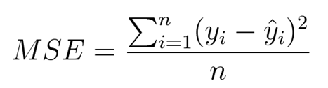
This expression can be defined as the mean value of the squared deviations of the predicted values from that of true values. Here ‘n’ denotes the total number of samples in the data.

Mean Absolute Error

Absolute Error for each training example is the distance between the predicted and the actual values, irrespective of the sign.

MAE = | y-f(x) |

Absolute Error is also known as the L1 loss. The MAE cost is more robust to outliers as compared to MSE.
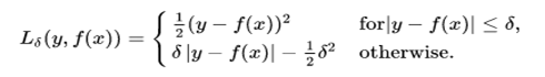
Huber Loss

Huber loss is a loss function used in robust regression. This is less sensitive to outliers in data than the squared error loss. The Huber loss function describes the penalty incurred by an estimation procedure f. Huber (1964) defines the loss function piecewise by:

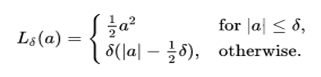
This function is quadratic for small values of a, and linear for large values, with equal values and slopes of the different sections at the two points where |a|= 𝛿. The variable “a” often refers to the residuals, that is to the difference between the observed and predicted values a=y-f(x), so the former can be expanded to: –

Binary Classification Loss Functions

Binary classifications are those predictive modelling problems where examples are assigned one of two labels.

Binary Cross-Entropy

Cross-Entropy is the loss function used for binary classification problems. It is intended for use with binary classification.

Mathematically, it is the preferred loss function under the inference framework of maximum likelihood. Cross-entropy will calculate a score that summarizes the average difference between the actual and predicted probability distributions for predicting class 1. The score is minimized and a perfect cross-entropy value is 0.

Hinge Loss

The hinge loss function is popular with Support Vector Machines (SVMs). These are used for training the classifiers,

l(y) = max(0, 1- t•y)

where ‘t’ is the intended output and ‘y’ is the classifier score.

Hinge loss is convex function but is not differentiable which reduces its options for minimizing with few methods.

Multi-Class Classification Loss Functions

Multi-Class classifications are those predictive modelling problems where examples are assigned one of more than two classes.

Multi-Class Cross-Entropy

Cross-Entropy is the loss function used for multi-class classification problems. It is intended for use with multi-class classification.

Mathematically, it is the preferred loss function under the inference framework of maximum likelihood. Cross-entropy will calculate a score that summarizes the average difference between the actual and predicted probability distributions for all classes. The score is minimized and a perfect cross-entropy value is 0.

Kullback Leibler Divergence Loss

KL divergence is a natural way to measure the difference between two probability distributions.

A KL divergence loss of 0 suggests the distributions are identical. In practice, the behaviour of KL Divergence is very similar to cross-entropy. It calculates how much information is lost (in terms of bits) if the predicted probability distribution is used to approximate the desired target probability distribution.

There are also some advanced loss functions for machine learning models which are used for specific purposes.

  1. Robust Bi-Tempered Logistic Loss based on Bregman Divergences
  2. Minimax loss for GANs
  3. Focal Loss for Dense Object Detection
  4. Intersection over Union (IoU)-balanced Loss Functions for Single-stage Object Detection
  5. Boundary loss for highly unbalanced segmentation
  6. Perceptual Loss Function

Robust Bi-Tempered Logistic Loss based on Bregman Divergences

In this loss function, we introduce a temperature into the exponential function and replace the softmax output layer of the neural networks by a high-temperature generalization. Similarly, the logarithm in the loss we use for training is replaced by a low-temperature logarithm. By tuning the two temperatures, we create loss functions that are non-convex already in the single-layer case. When replacing the last layer of the neural networks by our bi-temperature generalization of the logistic loss, the training becomes more robust to noise. We visualize the effect of tuning the two temperatures in a simple setting and show the efficacy of our method on large datasets. Our methodology is based on Bregman divergences and is superior to a related two-temperature method that uses the Tsallis divergence.

Minimax loss for GANs

Minimax GAN loss refers to the minimax simultaneous optimization of the discriminator and generator models.

Minimax refers to an optimization strategy in two-player turn-based games for minimizing the loss or cost for the worst case of the other player.

For the GAN, the generator and discriminator are the two players and take turns involving updates to their model weights. The min and max refer to the minimization of the generator loss and the maximization of the discriminator’s loss.

Focal Loss for Dense Object Detection

The Focal Loss is designed to address the one-stage object detection scenario in which there is an extreme imbalance between foreground and background classes during training (e.g., 1:1000). Therefore, the classifier gets more negative samples (or more easy training samples to be more specific) compared to positive samples, thereby causing more biased learning.

The large class imbalance encountered during the training of dense detectors overwhelms the cross-entropy loss. Easily classified negatives comprise the majority of the loss and dominate the gradient. While the weighting factor (alpha) balances the importance of positive/negative examples, it does not differentiate between easy/hard examples. Instead, we propose to reshape the loss function to down-weight easy examples and thus, focus training on hard negatives. More formally, we propose to add a modulating factor (1 − pt) γ to the cross-entropy loss, with tunable focusing parameter γ ≥ 0. 

We define the focal loss as

FL(pt) = −(1 − pt) γ log(pt)


Intersection over Union (IoU)-balanced Loss Functions for Single-stage Object Detection

The IoU-balanced classification loss focuses on positive scenarios with high IoU can increase the correlation between classification and the task of localization. The loss aims at decreasing the gradient of the examples with low IoU and increasing the gradient of examples with high IoU. This increases the localization accuracy of models.

Boundary loss for highly unbalanced segmentation

Boundary loss takes the form of a distance metric on the space of contours (or shapes), not regions. This can mitigate the difficulties of regional losses in the context of highly unbalanced segmentation problems because it uses integrals over the boundary (interface) between regions instead of unbalanced integrals over regions. Furthermore, a boundary loss provides information that is complementary to regional losses. Unfortunately, it is not straightforward to represent the boundary points corresponding to the regional softmax outputs of a CNN. Our boundary loss is inspired by discrete (graph-based) optimization techniques for computing gradient flows of curve evolution.

Following an integral approach for computing boundary variations, we express a non-symmetric L2L2 distance on the space of shapes as a regional integral, which avoids completely local differential computations involving contour points. This yields a boundary loss expressed with the regional softmax probability outputs of the network, which can be easily combined with standard regional losses and implemented with any existing deep network architecture for N-D segmentation. We report comprehensive evaluations on two benchmark datasets corresponding to difficult, highly unbalanced problems: the ischemic stroke lesion (ISLES) and white matter hyperintensities (WMH). Used in conjunction with the region-based generalized Dice loss (GDL), our boundary loss improves performance significantly compared to GDL alone, reaching up to 8% improvement in Dice score and 10% improvement in Hausdorff score. It also yielded a more stable learning process.

Perceptual Loss Function

We consider image transformation problems, where an input image is transformed into an output image. Recent methods for such problems typically train feed-forward convolutional neural networks using a \emph{per-pixel} loss between the output and ground-truth images. Parallel work has shown that high-quality images can be generated by defining and optimizing \emph{perceptual} loss functions based on high-level features extracted from pre-trained networks. We combine the benefits of both approaches and propose the use of perceptual loss functions for training feed-forward networks for image transformation tasks. We show results on image style transfer, where a feed-forward network is trained to solve the optimization problem proposed by Gatys et al in real-time. Compared to the optimization-based method, our network gives similar qualitative results but is three orders of magnitude faster. We also experiment with single-image super-resolution, where replacing a per-pixel loss with a perceptual loss gives visually pleasing results.

Conclusion

Loss function takes the algorithm from theoretical to practical and transforms neural networks from matrix multiplication into deep learning. In this article, initially, we understood how loss functions work and then, we went on to explore a comprehensive list of loss functions also we have seen the very recent — advanced loss functions.

References: –
 
https://arxiv.org
https://www.wikipedia.org
 

Interested in a career in Data Analyst?

To learn more about Data Analyst with Advanced excel course – Enrol Now.
To learn more about Data Analyst with R Course – Enrol Now.
To learn more about Big Data Course – Enrol Now.

To learn more about Machine Learning Using Python and Spark – Enrol Now.
To learn more about Data Analyst with SAS Course – Enrol Now.
To learn more about Data Analyst with Apache Spark Course – Enrol Now.
To learn more about Data Analyst with Market Risk Analytics and Modelling Course – Enrol Now.

A Step-by-Step Guide on Python Variables

A Step-by-Step Guide on Python Variables

Variable is the name given to the memory location where data is stored. Once a variable is stored, space is allocated in memory. Variables are named locations that are used to store references to the object stored in memory.

With the rapid rise of the advanced programming techniques, matching with the pacing advancements of Machine Learning and Artificial Intelligence, the need for Python for Data Analysis an Machine Learning Using Python is growing. However, when it comes to trustworthy courses, it is better to go for the best Python Certification Training in Delhi.

Now, coming to this article, here are some of the topics that will be covered in this article:

  • Rules to Define a Variable
  • Assigning Values to a Variable
  • Re-declaring a Variable in Python
  • Variable Scope
  • Deleting a Variable

Data Science Machine Learning Certification

Rules to Define a Variable

These are the few rules to define a python variable:

  1. Python variable name can contain small case letters (a-z), upper case letters (A-Z), numbers (0-9), and underscore (_).
  2. A variable name can’t start with a number.
  3. We can’t use reserved keywords as a variable name.
  4. The variable name can be of any length.
  5. Python variable can’t contain only digits.
  6. The variable names are case sensitive.

Assigning Values to a Variable

There is no need for an explicit declaration to reserve memory. The assignment is done using the equal to (=) operator.

Multiple Assignment in Python

Multiple variables can be assigned to the same variable.

Multi-value Assignment in Python

Multiple variables can be assigned to multiple objects.

Re-declaring a Variable in Python

After declaring a variable, one can again declare it and assign a new value to it. Python interpreter discards the old value and only considers the new value. The type of the new value can be different than the type of the old value.

Variable Scope

A variable scope defines the area of accessibility of the variable in the program. A Python variable has two scopes:

  1. Local Scope
  2. Global Scope

Python Local Variable

When a variable is defined inside a function or a class, then it’s accessible only inside it. They are called local variables and their scope is only limited to that function or class boundary.

If we try to access a local variable outside its scope, we get an error that the variable is not defined.

Python Global Variable

When the variable is not inside a function or a class, it’s accessible from anywhere in the program. These variables are called global variables.

Deleting a Variable

One can delete variable using the command “del”.

In the example below, the variable “d” is deleted by using command Del and when it is further proceeded to print, we get an error “variable name is not defined” which means the variable is already deleted.

Conclusion

In this article we have learned the concepts of Python variables which are used in every program. We also learned the rules associated to the naming of a variable, assigning value to a variable, scope of a variable and deleting a variable.

So, if you are also hooked into Python and looking for the best courses, Python course in Gurgaon is certainly a gem of a course!


This technical blog is sourced from: www.askpython.com and intellipaat.com


Interested in a career in Data Analyst?

To learn more about Data Analyst with Advanced excel course – Enrol Now.
To learn more about Data Analyst with R Course – Enrol Now.
To learn more about Big Data Course – Enrol Now.

To learn more about Machine Learning Using Python and Spark – Enrol Now.
To learn more about Data Analyst with SAS Course – Enrol Now.
To learn more about Data Analyst with Apache Spark Course – Enrol Now.
To learn more about Data Analyst with Market Risk Analytics and Modelling Course – Enrol Now.

An In-depth Analysis of Game Theory for AI

An In-depth Analysis of Game Theory for AI

Game Theory is a branch of mathematics used to model the strategic interaction between different players in a context with predefined rules and outcomes. With the rapid rise of AI, along with the extensive time and research we are devoting to it, Game Theory is experiencing steady growth. If you are also interested in AI and want to be well-versed with it, then, opt for the Best Artificial Intelligence Training Institute in Gurgaon now!

Games have been one of the main areas of focus in artificial intelligence research. They often have simple rules that are easy to understand and train for. It is clear when one party wins, and frankly, it is fun watching a robot beat a human at chess. This trend of AI research being directed towards games is not at all an accident. Researchers know that the underlying principles of many tasks lie in understanding and mastering game theory. Both AI and game theory seek to find out how participants will react in different situations, figuring out the best response to situations, optimizing auction prices and finding market-clearing prices.

Some Useful Terms in Game Theory

  • Game: Like games in popular understanding, it can be any setting where players take actions and its outcome will depend on them.
  • Player: A strategic decision-maker within a game.
  • Strategy: A complete plan of actions a player will take, given the set of circumstances that might arise within the game.
  • Payoff: The gain a player receives from arriving at a particular outcome of a game.
  • Equilibrium: The point in a game where both players have made their decisions and an outcome is reached.
  • Dominant Strategy: When one strategy is better than another strategy for one player, regardless of the opponent’s play, the better strategy is known as a dominant strategy.
  • Agent: Agent is equivalent to a player.
  • Reward: A payoff of a game can also be termed as a reward.
  • State: All the information necessary to describe the situation an agent is in.
  • Action: Equivalent of a move in a game.
  • Policy: Similar to a strategy. It defines the action an agent will make when in particular states
  • Environment: Everything the agent interacts with during learning.

Different Types of Games in Game Theory

In the game theory, different types of games help in the analysis of different types of problems. The different types of games are formed based on number of players involved in a game, symmetry of the game, and cooperation among players.

Cooperative and Non-Cooperative Games

Cooperative games are the ones in which the players are convinced to adopt a particular strategy through negotiations and agreements between them.

Non-Cooperative games refer to the games in which the players decide on their strategy to maximize their profit. Non-cooperative games provide accurate results. This is because in non-cooperative games, a very deep analysis of a problem takes place.

Data Science Machine Learning Certification

Normal Form and Extensive Form Games

Normal form games refer to the description of the game in the form of a matrix. In other words, when the payoff and strategies of a game are represented in a tabular form, it is termed as normal form games.

Extensive form games are the ones in which the description of the game is done in the form of a decision tree. Extensive form games help in the representation of events that can occur by chance.

Simultaneous Move Games and Sequential Move Games

Simultaneous games are the ones in which the move of two players (the strategy adopted by two players) is simultaneous. In a simultaneous move, players do not know the move of other players.

Sequential games are the ones in which the players do not have a deep knowledge about the strategies of other players.

Constant Sum, Zero Sum, and Non-Zero Sum Games

Constant sum games are the ones in which the sum of outcome of all the players remains constant even if the outcomes are different. 

Zero sum games are the ones in which the gain of one player is always equal to the loss of the other player. 

Non-zero sum games can be transformed to zero sum game by adding one dummy player. The losses of the dummy player are overridden by the net earnings of players. Examples of zero sum games are chess and gambling. In these games, the gain of one player results in the loss of the other player.

Symmetric and Asymmetric Games

Symmetric games are the ones where the strategies adopted by all the players are the same. Symmetry can exist in short-term games only because in long-term games the number of options with a player increases. 

Asymmetric games are the ones where the strategies adopted by players are different. In asymmetric games, the strategy that provides benefit to one player may not be equally beneficial for the other player.

Game Theory in Artificial Intelligence

Development of the majority of the popular games which we play in this digital world is with the help of AI and game theory. Game theory is used in AI whenever there is more than one person involved in solving a logical problem. There are various algorithms of Artificial Intelligence which are used in Game Theory. Minimax algorithm in Game Theory is one of the oldest algorithms in AI and is used generally for two players. Also, game theory is not only restricted to games but also relevant to the other large applications of AI like GANs (Generative Adversarial Networks).

GANs (Generative Adversarial Networks)

GAN consists of 2 models, a discriminative model and a generative model. These models are participants on the training phase which looks like a game between them, and each model tries to better than the other.

The target of the generative model is to generate samples that are considered to be fake and are supposed to have the same distribution of the original data samples; on the other hand, the target of discriminative is to enhance itself to be able to recognize the real samples among the fake samples generated by the generative model.

It looks like a game, in which each player (model) tries to be better than the other, the generative model tries to generate samples that deceive and tricks the discriminative model, while the discriminative model tries to get better in recognizing the real data and avoid the fake samples. It is the same idea of the Minimax algorithm, in which each player targets to outclass the other and minimize the supposed loss.

This game continues until a state where each model becomes an expert on what it is doing. The generative model increases its ability to get the actual data distribution and produces data like it, and the discriminative becomes an expert in identifying the real samples, which increases the system’s classification task. In such a case, each model satisfied by its output (strategy), this is called Nash Equilibrium in Game Theory.

Nash Equilibrium

Nash equilibrium, named after Nobel winning economist, John Nash, is a solution to a game involving two or more players who want the best outcome for themselves and must take the actions of others into account. When Nash equilibrium is reached, players cannot improve their payoff by independently changing their strategy. This means that it is the best strategy assuming the other has chosen a strategy and will not change it. For example, in the Prisoner’s Dilemma game, confessing is Nash equilibrium because it is the best outcome, taking into account the likely actions of others.

Conclusion

So in this article, the fundamentals of Game Theory and essential topics are covered in brief. Also, this article gives an idea of the influence of game theory artefacts in the AI space and how Game Theory is being used in the field of Machine Learning and its real-world implementations.

Machine Learning is an ever-expanding application of Artificial Intelligence with numerous applications in the other existing fields. Besides, Machine Learning Using Python is also on the verge of proving itself to be a foolproof technology in the coming years. So, don’t wait and enrol in the world-class Artificial Intelligence Certification in Delhi NCR now and rest assured! 


Interested in a career in Data Analyst?

To learn more about Data Analyst with Advanced excel course – Enrol Now.
To learn more about Data Analyst with R Course – Enrol Now.
To learn more about Big Data Course – Enrol Now.

To learn more about Machine Learning Using Python and Spark – Enrol Now.
To learn more about Data Analyst with SAS Course – Enrol Now.
To learn more about Data Analyst with Apache Spark Course – Enrol Now.
To learn more about Data Analyst with Market Risk Analytics and Modelling Course – Enrol Now.

Statistical Application in R & Python: Negative Binomial Distribution

Statistical Application in R & Python: Negative Binomial Distribution

Negative binomial distribution is a special case of Binomial distribution. If you haven’t checked the Exponential Distribution, then read through the Statistical Application in R & Python: EXPONENTIAL DISTRIBUTION.

It is important to know that the Negative Binomial distribution could be of two different types, i.e. – Type 1 and Type 2. In many ways, it could be seen as a generalization of the geometric distribution. The Negative Binomial Distribution essentially operates on the same principals as the binomial distribution but the objective of the former is to model for the success of an event happening in “n” number of trials. Here it is worth observing that the Geometric distribution models for the first success whereas a Negative Binomial distribution models for the Kth 

Data Science Machine Learning Certification

This is explained below.

Type 1 Binomial distribution  aims to model the trails up to and including the “kth success” in “n number of trials”. To give a simple example, imagine you are asked to predict the probability that the fourth person to hear a gossip will believe that! This kind of prediction could be made using the negative binomial type 1 distribution. 

Conversely, Type 2 Binomial distribution is used to model the number of failures before the “kth success”. To give an example, imagine you are asked about how many penalty kicks it will take before a goal is scored by a particular football player. This could be modeled using a negative binomial type 2 distribution, which might be pretty tricky or almost impossible with any other methods.

The probability distribution function is given below: 

In the next section, we will take you through its practical application in Python and R. 

Application:

Mr. Singh works in an Insurance Company where his target is to sale a minimum of five policies in a day. On a particular day, he had already sold 2 policies after numerous attempts. The probability of sales on each policy is 0.6. Now, if the policies may be considered as independent Bernoulli trials, then:

  1. What is the probability that he has exactly 4 failed attempts before his 3rd successful sales of the day?
  2. What is the probability that he was fewer than 4 failed attempts before his 3rd successful sales of the day?

So, the number of sales = 3.

The probability of failed attempts is 4.

The success of each sale is 0.6.

Calculate Negative Binomial Distribution in R:

In R, we calculate negative binomial distribution to find the probability of insurance sales. Thus, we get,

  1. The probability that he has exactly 4 failed attempts before his 3rd successful sales are 8.29%.
  2. The probability that he has fewer than 4 failed attempts before his 3rd successful sales is 82.08%.

Hence, we can see that chances are quite high that Mr. Singh will succeed in making a sale after 4 failed attempts.

Calculate Negative Binomial Distribution in Python:

In Python, we get the same results as above.

Conclusion:

Negative Binomial distribution is the discrete probability distribution that is actually used for calculating the success and failure of any observation. When applied to real-world problems, the outcomes of the successes and failures may or may not be the outcomes we ordinarily view as good and bad, respectively.

Suppose we used the negative binomial distribution to model the number of days a certain machine works before it breaks down. In this case, “success” would be the days that the machine worked properly, whereas the day when the machine breaks down would be a “failure”. Another example would be, if we used the negative binomial distribution to model the number of attempts an athlete makes on goal before scoring r goals, though, then each unsuccessful attempt would be a “success”, and scoring a goal would be “failure”.

This blog will surely aid in developing a better understanding of how negative binomial distribution works in practice. If you have any comments please leave them below. Besides, if you are interested in catching up with the cutting edge technologies, then reach the premium training institute of Data Science and Machine Learning leading the market with the top-notch Machine Learning course in India.


Interested in a career in Data Analyst?

To learn more about Data Analyst with Advanced excel course – Enrol Now.
To learn more about Data Analyst with R Course – Enrol Now.
To learn more about Big Data Course – Enrol Now.

To learn more about Machine Learning Using Python and Spark – Enrol Now.
To learn more about Data Analyst with SAS Course – Enrol Now.
To learn more about Data Analyst with Apache Spark Course – Enrol Now.
To learn more about Data Analyst with Market Risk Analytics and Modelling Course – Enrol Now.

How to Structure Python Programs? An Extensive Guide

How to Structure Python Programs? An Extensive Guide

Python is an extremely readable and versatile high-level programming language. It supports both Object-oriented programming as well as Functional programming. It is generally referred to as an interpreted language which means that each line of code is executed one by one and if the interpreter finds an error it stops proceeding further and gives an error message to the user. This makes Python a widely regarded language, fueling Machine Learning Using Python, Text Mining with Python course and more. Furthermore, with such a high-end programming language, Python for data analysis looks ahead for a bright future.

Data Science Machine Learning Certification

In the Structure of Python

Computer languages have a structure just like human languages. Therefore, even in Python, we have comments, variables, literals, operators, delimiters, and keywords.

To understand the program structure of Python we will look at the following in this article: –

  1. Python Statement
    • Simple Statement
    • Compound Statement
  2. Multiple Statements Per Line
  3. Line Continuation
    • Implicit Line Continuation
    • Explicit Line Continuation
  4. Comments
  5. Whitespace
  6. Indentation
  7. Conclusion

Python Statement

A statement in Python is a logical instruction that the interpreter reads and executes. The interpreter executes statements sequentially, one by one. In Python, it could be an assignment statement or an expression. The statements are mostly written in such a style so that each statement occupies a single line.

Simple Statements

A simple statement is one that contains no other statements. Therefore, it lies entirely within a logical line. An assignment is a simple statement that assigns values to variables, unlike in some other languages; an assignment in Python is a statement and can never be part of an expression.

Compound Statement

A compound statement contains one or more other statements and controls their execution. A compound statement has one or more clauses, aligned at the same indentation. Each clause has a header starting with a keyword and ending with a colon (:), followed by a body, which is a sequence of one or more statements. When the body contains multiple statements, also known as blocks, these statements should be placed on separate logical lines after the header line, indented four spaces rightward.

Multiple Statements per Line

Although it is not considered good practice multiple statements can be written in a single line in Python. It is advisable to avoid multiple statements in a single line. But, if it is necessary, then it can be written with the help of semicolon (;) as the terminator of every statement.

Line Continuation

In Python there might be some cases when a single statement is too long that does not fit the browser window and one needs to scroll the screen left or right. This can be a case of assignment statement with many terms or defining a lengthy nested list. These long statements of code are generally considered a poor practice.

To maintain readability, it is advisable to split the long statement into parts across several lines. In Python code, a statement can be continued from one line to the next in two different ways: implicit and explicit line continuation.

Implicit Line Continuation

This is the more straightforward technique for line continuation. In implicit line continuation, one can split a statement using either of parentheses ( ), brackets [ ] and braces { }. Here, one needs to enclose the target statement using the mentioned construct.

Explicit Line Continuation

In cases where implicit line continuation is not readily available or practicable, there is another option. This is referred to as an explicit line continuation or explicit line joining. Here, one can right away use the line continuation character (\) to split a statement into multiple lines.

Comments

A comment is text that doesn’t affect the outcome of a code; it is just a piece of text to let someone know what you have done in a program or what is being done in a block of code. This is especially helpful when a code is written and someone is analyzing it for bug fixing or making a change in logic, by reading a comment one can understand the purpose of code much faster than by just going through the actual code.

There are two types of comments in Python.
1. Single line comment
2. Multiple line comment

Single line comment

In python, one can use # special character to start the comment.

Multi-line comment

To have a multi-line comment in Python, one can use Triple Double Quotation at the beginning and the end of the comment.

Whitespace

One can improve the readability of the code with the use of whitespaces. Whitespaces are necessary for separating the keywords from the variables or other keywords. Whitespace is mostly ignored by the Python interpreter.

Indentation

Most of the programming languages provide indentation for better code formatting and don’t enforce to have it. However, in Python, it is mandatory to obey the indentation rules. Typically, we indent each line by four spaces (or by the same amount) in a block of code. Also for creating compound statements, the indentation will be of utmost necessity.

Conclusion

So, this article was all about how to structure the Python program. Here, one can learn what constitutes a valid Python statement and how to use implicit and explicit line continuation to write a statement that spans multiple lines. Furthermore, one can also learn about commenting Python code, and about the use of whitespace and indentation to enhance the overall readability.

Our Machine Learning Certifications have undergone an industrial upgradation

We hope this article was helpful to y ou. If you are interested in similar blogs, stay glued to our website, and keep following all the news and updates from Dexlab Analytics.


Interested in a career in Data Analyst?

To learn more about Data Analyst with Advanced excel course – Enrol Now.
To learn more about Data Analyst with R Course – Enrol Now.
To learn more about Big Data Course – Enrol Now.

To learn more about Machine Learning Using Python and Spark – Enrol Now.
To learn more about Data Analyst with SAS Course – Enrol Now.
To learn more about Data Analyst with Apache Spark Course – Enrol Now.
To learn more about Data Analyst with Market Risk Analytics and Modelling Course – Enrol Now.

Statistical Application in R & Python: EXPONENTIAL DISTRIBUTION

Statistical Application in R & Python: EXPONENTIAL DISTRIBUTIONStatistical Application in R & Python: EXPONENTIAL DISTRIBUTION

In this blog, we will explore the Exponential distribution. We will begin by questioning the “why” behind the exponential distribution instead of just looking at its PDF formula to calculate probabilities. If we can understand the “why” behind every distribution, we will have a head start in figuring out its practical uses in our everyday business situations.

Much could be said about the Exponential distribution. It is an important distribution used quite frequently in data science and analytics. Besides, it is also a continuous distribution with one parameter “λ” (Lambda). Lambda as a parameter in the case of the exponential distribution represents the “rate of something”. Essentially, the exponential distribution is used to model the decay rate of something or “waiting times”.

Data Science Machine Learning Certification

For instance, you might be interested in predicting answers to the below-mentioned situations:

  • The amount of time until the customer finishes browsing and actually purchases something in your store (success).
  • The amount of time until the hardware on AWS EC2 fails (failure).
  • The amount of time you need to wait until the bus arrives (arrival).

In all of the above cases if we can estimate a robust value for the parameter lambda, then we can make the predictions using the probability density function for the distribution given below:

Application:-

Assume that a telemarketer spends on “average” roughly 5 minutes on a call. Imagine they are on a call right now. You are asked to find out the probability that this particular call will last for 3 minutes or less.


Below we have illustrated how to calculate this probability using Python and R.

Calculate Exponential Distribution in R:

In R we calculate exponential distribution and get the probability of mean call time of the tele-caller will be less than 3 minutes instead of 5 minutes for one call is 45.11%.This is to say that there is a fairly good chance for the call to end before it hits the 3 minute mark.

Calculate Exponential Distribution in Python:

We get the same result using Python.

Conclusion:

We use exponential distribution to predict the amount of waiting time until the next event (i.e., success, failure, arrival, etc).

Here we try to predict that the probability of the mean call time of the telemarketer will be less than 3 minutes instead of 5 minutes for one call, with the help of Exponential Distribution. Similarly, the exponential distribution is of particular relevance when faced with business problems that involve the continuous rate of decay of something. For instance, when attempting to model the rate with which the batteries will run out. 

Data Science & Machine Learning Certification

Hopefully, this blog has enabled you to gather a better understanding of the exponential distribution. For more such interesting blogs and useful insights into the technologies of the age, check out the best Analytics Training institute Gurgaon, with extensive Data Science Courses in Gurgaon and Data analyst course in Delhi NCR.

Lastly, let us know your opinions about this blog through your comments below and we will meet you with another blog in our series on data science blogs soon.


Interested in a career in Data Analyst?

To learn more about Data Analyst with Advanced excel course – Enrol Now.
To learn more about Data Analyst with R Course – Enrol Now.
To learn more about Big Data Course – Enrol Now.

To learn more about Machine Learning Using Python and Spark – Enrol Now.
To learn more about Data Analyst with SAS Course – Enrol Now.
To learn more about Data Analyst with Apache Spark Course – Enrol Now.
To learn more about Data Analyst with Market Risk Analytics and Modelling Course – Enrol Now.

Alteryx is Inclined to Make Things Easy

Alteryx is Inclined to Make Things Easy

Alteryx Analytics is primarily looking to ease the usability of the platform in all of the updates that are yet to come. The esteemed data analytics platform is concentrating on reducing the complexities to attract more users and thus, widen their age-old user base beyond that of the data scientists and data analytics professionals.

Alteryx is headquartered in Irvine, California. It was founded as SRC LLC in 1997 and comes with a suite of four tools to help the world of data scientists and data analysts to manage and interpret data easily. Alteryx Connect, Alteryx Designer, Alteryx Promote and Alteryx Server are the main components of the analytics platform of Alteryx. Thus, it is worth mentioning that the Alteryx Certification Course is a must if you are looking to make a career out of data science/data analytics.

Deep Learning and AI using Python

A Quick Glance at the Recent Updates 

The reputed firm launched a recent version of Alteryx 2019.3, in October, and is likely to release the Alteryx 2019.4 as a successor to it. The latter is scheduled for a December release.

What’s in the Update?

Talking about the all-new version Alteryx 2019.3, Ashley Kramer, senior vice president of product management at Alteryx, said that the latest version promises 25 new and upgraded features, all of them focussing on the user-friendliness of the platform at large.

One of the prominent features of the new version is a significant decrease in the total number of clicks that a user will take to arrive at the option of visualizing data to make analytic decisions.

Data profiling helps the users to visualize the data while they are working with it. Here, Alteryx discovered a painless way to work with data by modeling the bottom of the screen in a format similar to that of MS Excel.

All of these changes and additions are done keeping in mind the features that the “customers had been asking for,” according to Kramer.

Now, with the December update, which will come with an enhanced mapping tool, the Alteryx analytics will strive to further lower the difficulties surrounding the platform.

2

If you are interested in knowing all the latest features, it is better to join one of the finest AlterYX Training institutes in Delhi NCR, with exhaustive Analytics Courses in Delhi NCRalong with other demanding courses like Python for Data Analysis, R programming courses in Gurgaonmatchless course of Big Data, Data Analytics and more.

 
The blog has been sourced fromsearchbusinessanalytics.techtarget.com/news/252474294/Alteryx-analytics-platform-focuses-on-ease-of-use
 

Interested in a career in Data Analyst?

To learn more about Data Analyst with Advanced excel course – Enrol Now.
To learn more about Data Analyst with R Course – Enrol Now.
To learn more about Big Data Course – Enrol Now.

To learn more about Machine Learning Using Python and Spark – Enrol Now.
To learn more about Data Analyst with SAS Course – Enrol Now.
To learn more about Data Analyst with Apache Spark Course – Enrol Now.
To learn more about Data Analyst with Market Risk Analytics and Modelling Course – Enrol Now.

An All-Inclusive Guide on Python and its Changing Trends

An All-Inclusive Guide on Python and its Changing Trends

Python is an extremely readable and versatile high-level programming language. Many companies such as Google, YouTube, Dropbox use the language for developing applications. It also finds its use extensively in diverse fields as in Python for data analysis, Machine Learning Using Python, Natural Language Processing, Web Development, Scientific Computing, Image processing, Robotics, Computer Vision and many more.

It supports both Object-oriented programming and Functional programming. Python is generally referred to as an interpreted language which implies that each line of code is executed one by one and if the interpreter finds an error, it stops immediately with an error message on the screen.

Another important feature of Python is its interactive prompt. A Python statement can be typed and immediately executed, which is in sharp contradiction to any other compiled language.

What are Python 2.x and Python 3.x?

There are two main versions of Python: Python 2.x and Python 3.x. If someone is new to Python, then he/she might be in confusion about which version to use. However, in the current scenario, we can easily migrate from Python 2 to Python 3, as the Python Software Foundation has finally taken the step to formally announce that Python 2 will reach the end of life (EOL) on January 1st, 2020.

Key differences between Python 2.x and Python 3.x

This article discusses the differences between these two versions of Python, making Python 3 less confusing for a new programmer.

  1. Print Function

In Python 2, print is a statement. There is no need of parenthesis.

In Python 3, print is a function. It needs parenthesis.

  1. Integer Division

In Python 2, if the division operator is performed on two integers, then the output will be an integer for example: – 7/3 = 2.

In Python 3, if the division operator is performed on two integers, then the output will be accurate. It can also be in float for example: – 7/3 = 2.33.

To get the result in an integer only a different division operator is used that is (//) it returns an integer result for example, – 7//3 = 2.

 3. Unicode Support

Both the versions of Python can handle strings (sequences of characters) differently.

Python 2 uses the ASCII encoding standard by default. ASCII is limited to representing 256 characters. This limits the flexibility of Python to encode the characters, particularly non-standard ones. Using Unicode in Python 2 requires extra syntax—for example when using print, the input text is to be wrapped in the Unicode() function to handle special characters.

In Python 3, Unicode is the default. The Unicode standard is much more versatile—it supports over 128,000 characters. There is no need for an extra syntax to define the Unicode values—they get printed automatically as utf-8 strings.

  1. Range Function

In Python 2, the range function returns a list of numbers.

In Python 2, the xrange class represents an iterable that provides the same object.

 In Python 3, original range function is removed and xrange is renamed to range:

In Python 3, it is needed to convert the range object to a list if someone desires the same result as the range function provides in Python 2.

  1. ­­­­Input() Method

Mainly what is expected from the input() method is that it reads input as string, then it can be converted into any datatype as per the requirement.

In Python 2, it has both the input() and raw_input() methods for taking input. The difference between the raw_input() and input()is that the raw_input() reads input as a string while the input() reads input as string only if it is inside quotes else reads as an integer.

In Python 3, there is no raw_input() method. The raw_input() method is replaced by input() in python 3. 

If someone still wants to use the input() method like in python 2, then it can be availed by using eval() method.

There are many other differences between Python 2 and Python 3 like: –

  1. Next() Method

In Python 2, .next() method is used and in Python 3 next() function is used to iterate the next element of an iterator.

  1. Raising Exception

To raise an exception in Python 3, the argument should be in parenthesis, while in Python 2, it is not necessary.

  1. Handling Exception

Handling exception is also changed in Python 3, “as” keyword is used in Python 3, while it is not necessary in Python 2.

So, if someone is a beginner, then it is strongly recommended to use Python 3 because it is the future of Python and also January 1, 2020, will be the last day of Python 2. It means that no improvement will be done anymore after that day, even if someone finds a security problem in it.

Data Science Machine Learning Certification

It is highly recommended to upgrade the version of the programming language to Python 3. Some ways can help the Python 2 users in porting their code from Python 2 to Python 3 and get the feel of Python 3 and figure out how it is different from Python 2. The code can be imported by using tools like “Futurize” and “Modernize”. Also, if someone wants to check the availability of Python 3 as part of his tests, then “caniusepython3.check()” can be used.

As a final note, everyone must look for upgrading their Python version to Python 3 to understand the subtleties of the new version and usher in the future. However, if you are interested in Deep learning for computer vision with Python and similar courses, then opt for the premium Python training institute in Delhi now!


.

8 Amazing Things That Artificial Intelligence Can Do

8 Amazing Things That Artificial Intelligence Can Do

AI plays a crucial role in our everyday lives. By now, we are aware of AI’s glaring significance in our very existence. Nevertheless, you would be surprised to know that AI has already imbibed some of the skills that we, humans, possess. Ahead, we’ve 8 incredible skills that AI has learnt over the years:

Read

Wondering how to summarize all those kilobytes of information? AI-powered SummarizeBot is the answer. Whether its books, news articles, weblinks, audio/image files or legal documents, ATS (automatic text summarization) reads everything and records the important information. Natural Language Processing (NLP), artificial intelligence, machine learning and blockchain technologies are in play here.  

2

Write

Did you know that myriad news enterprises and seasoned journalists rely on AI to write? The New York Times, Reuters, Washington Post and more have turned to artificial intelligence to craft interesting reading pieces. Also, AI is expected to enhance the process of creative writing as well.  Even, it has generated a novel that was shortlisted for a prestigious award.

See

Machine vision is in the hype. It is implemented in different ways in today’s world, such as facilitating self-driven cars, facial recognition for payment portals, police work and more. The main concept of machine vision is to let the computers ‘visualize’ the world, analyze key data and make decisions thereafter.

Speak

We are fortunate enough to have Google Maps and Alexa to give us directions and respond to our queries but Google Duplex takes it to a whole new level, courtesy AI. With the help of this robust technology, Duplex can schedule appointments and finish tasks on phone in a very interactive language. It can also respond perfectly to human behaviors.

Hear and Understand

Detecting gunshots and alerting to-the-purpose agencies is one of the greatest things achieved by AI. It means AI can hear and understand sound. It is very well evident in how digital voice assistants respond to your queries regarding weather or a day’s agenda. Working professionals simply love the efficiency, accuracy and convenience of automated meeting minutes provided by AI.

Touch

With the help of cameras and sensors, a robot can identify and handpick ‘supermarket ripe’ blueberries and put them in your basket. The creator of the robot even asserts that it is designed to pick one blueberry every 10 seconds for 24 hours a day!

Deep Learning and AI using Python

Smell

A team of AI researchers are at present developing robust AI models that can detect illnesses – simply by smelling. The model is designed in such a way so that it can notice chemicals, known as aldehydes that cause human stress and diseases, including diabetes, cancer and brain injuries. AI bots can even identify other caustic chemicals or gas leaks. Of late, IBM is using AI to formulate new perfumes.

Perceive Emotions

Today, AI tools can observe human emotions and track them down as one watches videos. Artificial emotional intelligence can collect meaningful data from a person’s facial expressions or body language, analyze it to determine what emotion he/she is likely to express and then ascertain an action base on that detail.

For more such interesting updates, follow DexLab Analytics. Our Machine Learning Using Python course is a bestseller. To know more, click here <www.dexlabanalytics.com>


This post originally appeared onwww.forbes.com/sites/bernardmarr/2019/11/11/13-mind-blowing-things-artificial-intelligence-can-already-do-today/#2777e5ec6502


Interested in a career in Data Analyst?

To learn more about Data Analyst with Advanced excel course – Enrol Now.
To learn more about Data Analyst with R Course – Enrol Now.
To learn more about Big Data Course – Enrol Now.

To learn more about Machine Learning Using Python and Spark – Enrol Now.
To learn more about Data Analyst with SAS Course – Enrol Now.
To learn more about Data Analyst with Apache Spark Course – Enrol Now.
To learn more about Data Analyst with Market Risk Analytics and Modelling Course – Enrol Now.

Call us to know more