python course in Gurgaon Archives - Page 3 of 9 - DexLab Analytics | Big Data Hadoop SAS R Analytics Predictive Modeling & Excel VBA

Visualization with Python Part III: Introducing The Seaborn Library

Posted on September 1, 2020September 1, 2020 by Dexlab

In this 3rd part of the visualization series using Python programming language, we are going to introduce you to the Seaborn Library. Seaborn is a visualization library which is built on top of Matplotlib library in Python. This library helps us build method based plots which when combined with Matplotlib library methods lets us build flexible graphs.

In this tutorial we will be using tips data, which is a pre-defined dataset in the Seaborn library.

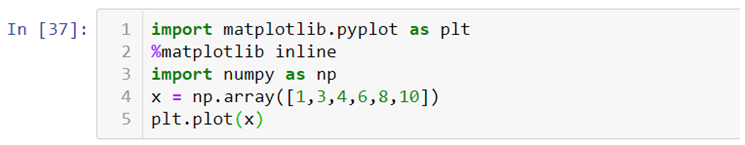
So let’s begin by importing the Seaborn library and giving it a sudo name sns. We will also be importing Matplotlib library to add more attributes to our graphs.

To load the tips data set we will be using .load_dataset() method.

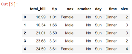
Data description:- This is a dataset of a restaurant which keeps a record of the amount of bill paid by a customer, tip amount over the total bill paid, gender of the customer, whether he or she was a smoker or not, the day on which they ate at the restaurant, what was the time when they ate at the restaurant and the size of the table they booked.

In case while loading the dataset you see a warning box appear on the screen you don’t need to worry , you haven’t done anything wrong. These FutureWarning boxes appear to make you aware that in the future there might be some changes in the library or methods you are using.

You can simply use the .simplefilter() method from the warning library to make them disappear.

Here the category argument helps you decide which type of warning you want to ignore.

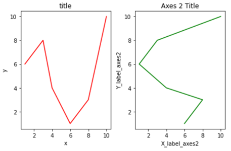
Creating a bar plot in Seaborn

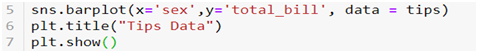
Now let’s quickly go ahead and create a bar plot with the help of .barplot() method.

In the above line of code we are using column named sex on the x axis and total_bill on the y axis. But this bar plot is very different from the bar plot which we usually make. The basic concept of a bar plot is to check the frequency but here we are also mentioning the y axis data which in general is not the case with a normal bar plot, that is, we get the frequency on the y axis when we are plotting a bar graph. So what does the above code do?

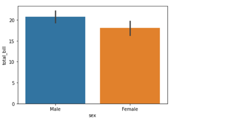
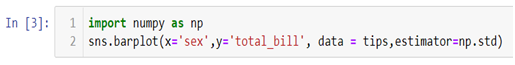
The above code compares the average of the category. In our case the above graph shows that the average bill of male is higher than the average bill of female. In case you want to plot a graph showing the average variation of bill around the mean (Standard deviation) you can use estimator argument within the .barplot() to do so.

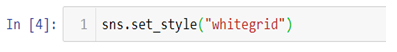
Also if you want to change the background of your graph you can easily do so by using .set_style() method.

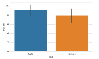
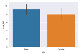
The vertical bars between the graph are called the error bars and they tell you how far from your mean or standard deviation by max data varies.

How to add Matplotlib attributes to your Seaborn graphs

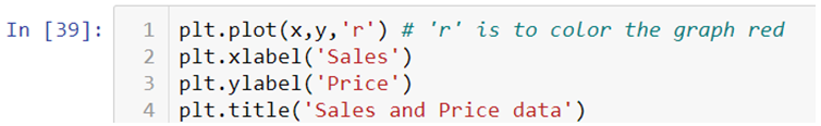
Matplotlib methods can be imported and added to the Seaborn graphs to make them more presentable and flexible. Here we will be adding a title in our graph by using .title() method from the Matplotlib library.

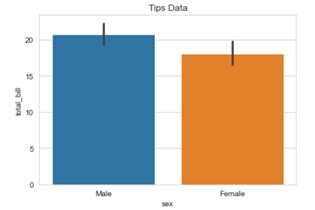
You can use other Matplotlib methods like .legend(),xlabel(),.ylabel() etc,. to add more value to your graphs.

The video tutorial attached below will further help you clarify your ideas regarding the Seaborn library. Follow the series to gain expertise in visualization with Python programming language. Keep on following the Dexlab Analytics blog for reading more informative posts on Python for data science training.

An Introduction to Matplotlib Object Oriented Method: Visualization with Python (Part II)

Posted on August 31, 2020August 31, 2020 by Dexlab

In the last blog that covered Part 1 of the visualization series using Python programming language, we have learned the basics of the Matplotlib Library. Now that our grasp on the basics is strong we would move further. Let’s break it all down with a more formal introduction of Matplotlib’s Object Oriented API. This means we will instantiate figure objects and then call methods or attributes from that object.

Introduction to the Object Oriented Method

The main idea in using the more formal Object Oriented method is to create figure objects and then just call methods or attributes off of that object. This approach is nicer when dealing with a canvas that has multiple plots on it.

How to make multiple plots using .add_axes()

To begin, we create a figure instance. Then we can add axes to that figure where .figure()is a method which helps us create an empty canvas and then we use .add_axes() method to give the position where the plot is to be made. The positional arguments [left, bottom, width, height] help us decide from where the graph should begin within the canvas and what should be the width and the height of the graph. Since the area of the graph is 100% (1.0), the range of the positional argument should be between 0 and 1 and in case you want to plot the graph half within and half outside the canvas, you can go beyond the specified range depending upon your needs.

Let’s quickly get to the coding part now.

In the above line of codes we are simply importing the Matplotlib library and creating a data which we want to plot.

plt.figure()method is helping us create an empty canvas and then we are giving the positional values to the .add_axes() method. As you can see we are using a variable named fig to save our canvas and then using the same variable as an object to add an axes to the canvas. Now all we need to do is use that axes to build are graph by adding x and y data.
Now you must be wondering why we aren’t able to see a plot in the corner of the canvas? It is because this procedure works only if we were to build multiple plots. So now let’s see how we can use the .add_axes() method to build multiple plots on top of each other.

In the above line of codes we are creating three axes and each axes is smaller than the other so that we are able to plot multiple graphs on top of each other.

Here we are making three different graphs and each graph has its own title and x axis and y axis labels. But to add title and axis labels we are now using .set_title(), .set_xlabel(), and .set_ylabel() instead of .title(), .xlabel() and .ylabel(). In axes2.plot() we are also using RGB color instead of using the predefined color in .plot() method. You can use your favorite color too by simply typing RGB color picker in your Google search and copy pasting the color code in the .plot() method. After running the above code we get the following graph:-

How to make multiple plots using .subplots()

.subplots() method is similar to the previous .subplot() method, the only difference is that now we use it on a canvas.

In the .subplots() we do not mention the plot number instead we use plot indexing method to build graph.
As you can see we are accessing the index number to build our plot and then using .tight_layout() method to keep the graphs from overlapping. After running the above code we get the following graphs:-

Do not forget to check out the video tutorial attached below to learn how this method works. Keep following the series to upgrade your skills and to explore more informative posts on topics like Python Programming training you need to follow the Dexlab Analytics blog.

A Quick Guide To Using Matplotlib Library (Part I)

Posted on August 27, 2020August 31, 2020 by Dexlab

Matplotlib is the “grandfather” library of data visualization with Python. It was created by John Hunter. He created it to try replicating MatLab’s (another programming language) plotting capabilities in Python. So, if you are already familiar with matlab, matplotlib will feel natural to you.

This library gives you the flexibility to plot the graphs the way you want. You can start with a blank canvas and plot the graph on that canvas wherever you want. You can make multiple plots on top of each other, change the line type, change the line color using predefined colors or hex codes, line width etc.

Installation

Before you begin you’ll need to install matplotlib first by using the following code:-

There are two ways in which you can built matplotlib graphs:-

Method based graphs
Object-oriented graphs

Method Based Graphs in Matplotlib:-

There are pre-defined methods in matplotlib library which you can use to create graphs directly using python language for example:-

Where, import matplotlib.pyplot as plt this code is used to import the library, %matplotlib inline is used to keep the plot within the parameters of the jupyter notebook, import numpy as np and x = np.array([1,3,4,6,8,10]) is used to import the numpy (numerical python) library and create an array x and plt.plot(x) is used to plot the distribution of the x variable.

We can also use .xlabel(), .ylabel() and .title() methods print x axis and y axis labels and title on the graph.

If you want to add text within your graph you can either use .annotate() method or .text() method.

Creating Multiplots

You can also create multiple plots by using .subplot() method by mentioning the number of rows and columns in which you want your graphs to be plotted. It works similar to the way you mention the number of rows and columns in a matrix.

You can add title, axis labels, texts etc., on each plot separately. In the end you can add .tight_layout() to solve the problem of overlapping of the graphs and to make the labels and scales visible.

Check out the video attached below to get an in-depth understanding of how Matplotlib works. This is a part of a visualization series using Python programming language. So, stay tuned for more updates. You can discover more such informative posts on the Dexlab Analytics blog.

Advertising Gets Smarter With Machine Learning

Posted on August 20, 2020August 20, 2020 by Dexlab

Every single day we get deluged by advertising messages in many formats. From your morning newspaper to Youtube to Facebook, there is hardly a platform left that is not getting utilized by smart marketers. After all, advertising is a powerful marketing tool with the power to sway opinions in favor or, against, and careful planning and placement play a crucial role in making an ad click with the target audience. The digital era has opened up multiple avenues for the advertisers but, it has also posed new challenges for them.

To stay ahead in the game advertisers have been quicker to recognize the potential of integrating advanced technology such as Machine Learning to optimize their ad campaigns. ML algorithms can process data and analyze patterns to offer predictions that in turn helps marketers fine-tune their marketing strategies.

Google AdWords is a case in point that has incorporated machine learning to leverage their ad game. Marketing professionals now should upskill themselves with Machine Learning course in Delhi, to ensure seamless integration of this technology into advertising.

How ML is benefiting the advertising industry?

ML can boost ad performance

Incorporating machine learning techniques can reduce the time, labor, and amount of error that go into processing data to identify factors that when tweaked could positively influence your ad performance. Machine learning not only automates the task but, also comes up with several solutions keeping your goal and budget in mind as well as other significant criteria. With time the more data get fed into the system the more accurate results could be expected.

Ad Creatives get better

Creative ads draw more attention, a catchy headline, slogan or, visual or, the combo of all these elements coupled with others contribute to making an ad a roaring success and in turn, boosting a product or brand image. Now, one might wonder what algorithms have to do with creative thinking which is completely a spontaneous affair, but, ML might be of help in here. Before investing money in designing creatives, use ML to assess past campaigns to measure all the elements and offer insight regarding imagery, color, font style, size, messages, and other factors. Furthermore, different personality types react differently to a given message, so gaining an insight into that behavior pattern is vital before delving into designing.

Be more relevant and relatable

Advertising is all about delivering the message to the targeted audience, but, instead of just sorting through random survey data to identify groups, using ML to go deeper into the process can create a big impact on the results. Using ML techniques social media interactions of people could be parsed to identify areas that interest them, people that influence them, and so on. Another factor that matters here is to identifying the right combination of time and platform to reach your target audience to make the maximum impact, ML algorithms enable you to do all of that.

Better segmentation

While designing any ad campaign, the marketer needs to identify the segment they are targeting. Instead of applying age-old methods that only scratch the surface, smart algorithms can dive in to help you be more specific about your segments and not just that but it could also identify that layer of audience hidden in the data who normally do not come under your segmentation, but has the potential to convert into paying customers if approached.

Predict campaign results

Implementation of ML can ensure that you get to test the success or, failure of your campaign even before it hits the viewers. Assessment of previous campaigns coupled with customer data using ML techniques can give you an idea regarding the performance of your campaign. It allows you to rectify or, revise any strategy that might sound or, look iffy. It can also help you make smart media buying decisions and point you towards platforms that you didn’t consider in the first place.

The field of advertising is deriving huge benefits from incorporating ML technology. However, choosing the right tool that works best for the specific needs of a campaign is essential. Another factor is having trained employees with a background in Machine Learning Using Python, is essential as they would be in charge of implementing and monitoring the technology.

Gradient Boosting In scikit-learn 0.22 For Handling Missing Values

Posted on August 10, 2020August 10, 2020 by Dexlab

A new tutorial session regarding the scikit-learn 0.22 is here and our sole focus is going to be updating your knowledge regarding the new features that have been added to this library. For this particular session we have decided to introduce you to the concept of gradient boosting that can handle the missing values. This concept is being introduced to clear out a previous misconception regarding the functioning of gradient boosting for this particular purpose.

The earlier notion surrounding GBM or, the gradient boosting algorithm in scikit-learn, was that it was unable to handle the missing values. In this tutorial we want to clarify that misconception, because, contrary to the notion XGBoost library or, XGB library is perfectly capable of handling the missing value analysis. It has been found that XGB library performs better than the normal method taken to find the missing values.

Now getting back to the scikit-learn 0.22 way of solving the issue of missing values. There has been an enhancement in the algorithm gradient boosting due to which you no longer have to handle the missing values because it will handle it of itself.

So take a look at how the concept of native support for missing values for gradient boosting works.

The ensemble algorithm, ensemble.HistGradientBoostingClassifier and ensemble.HistGradientBoostingRegressor, both classification regression now have the power of native support for missing values or, (NaNs). This is indicative of the fact that there is no need now for imputing data during training or predicting.

To gain an insight into how you perform this you need to follow the complete code sheet that you can find here

Now, as you go through the code you will find the word enable, which might surprise you and make you question why it says enable here? Well, this is because it is still being developed.

So, basically all of the algorithms in the scikit-learn 0.22 that are under development process have to run an extra line of code that goes like enable_hist_gradient_boosting. After further development there won’t be any need of that.

The video attached below will further explain how the algorithm works.

There will be more informative tutorial sessions like this, so to stay updated keep following the DexLab Analytics blog.

Watch the video here.

A Quick Guide to Data Mining

Posted on July 23, 2020July 23, 2020 by Dexlab

Data mining refers to processing mountainous amount of data that pile up, to detect patterns and offer useful insight to businesses to strategize better. The data in question could be both structured and unstructured datasets containing valuable information and which if and when processed using the right technique could lead towards solutions.

Enrolling in a Data analyst training institute, can help the professionals involved in this field hone their skills. Now that we have learned what data mining is, let’s have a look at the data mining techniques employed for refining data.

Data cleaning

Since the data we are talking about is mostly unstructured data it could be erroneous, corrupt data. So, before the data processing can even begin it is essential to rectify or, eliminate such data from the data sets and thus preparing the ground for the next phases of operations. Data cleaning enhances data quality and ensures faster processing of data to generate insight. Data Science training is essential to be familiar with the process of data mining.

Classification analysis

Classification analysis is a complicated data mining technique which basically is about data segmentation. To be more precise it is decided which category an observation might belong to. While working with various data different attributes of the data are analyzed and the class or, segments they belong to are identified, then using algorithms further information is extracted.

Regression analysis

Regression analysis basically refers to the method of deciding the correlation between variables. Using this method how one variable influences the other could be decided. It basically allows the data analyst to decide which variable is of importance and which could be left out. Regression analysis basically helps to predict.

Anomaly detection

Anomaly detection is the technique that detects data points, observations in a dataset, that deviate from an expected or, normal pattern or behavior. This anomaly could point to some fault or, could lead towards the discovery of an exception that might offer new potential. In fields like health monitoring, or security this could be invaluable.

Clustering

This data mining technique is somewhat similar to classification analysis, but, different in the way that here data objects are grouped together in a cluster. Now objects belonging to one particular cluster will share some common thread while they would be completely different from objects in other clusters. In this technique visual presentation of data is important, for profiling customers this technique comes in handy.

Association

This data mining technique is employed to find some hidden relationhip patterns among variables, mostly dependent variables belonging to a dataset. The recurring relationships of variables are taken into account in this process. This comes in handy in predicting customer behavior, such as when they shop what items are they likely to purchase together could be predicted.

Tracking patterns

This technique is especially useful while sorting out data for the businesses. In this process while working with big datasets, certain trends or, patterns are recognized and these patterns are then monitored to draw a conclusion. This pattern tracking technique could also aid in identifying some sort of anomaly in the dataset that might otherwise go undetected.

Big data is accumulating every day and the more efficiently the datasets get processed and sorted, the better would be the chances of businesses and other sectors be accurate in predicting trends and be prepared for it. The field of data science is full of opportunities now, learning Data science using python training could help the younger generation make it big in this field.

KNN Imputer – Release Highlights for Scikit-learn 0.22

Posted on July 1, 2020August 10, 2020 by Dexlab

Today we are going to learn about the new feature of Scikit-learn version 0.22 called KNN Imputation. This feature now enables us to support imputation for completing missing values using k-Nearest Neighbours (KNN). To track our tutorials on other new releases from scikit-learn, read our blog here and here.

Introduction

Each sample’s missing values are imputed using the mean value from nearest neighbours found in the training set. Two samples are close if the features that are neither missing are close. By default, a Euclidean distance metric that supports missing values, nan_euclidean_distances, is used to find the nearest neighbours.

Input and Output

So, what we do first is to import libraries like NumPy and run them. Then we create as many rows as we wish to. Then we run the function KNN Imputer and we can decide how many neighbours we want. We first, as is the procedure to use scikit-learn goes, create an object and then run it. Then we can directly put the input values in imputer.fit_transform and get the output values in the form of patterns detected in the input values.

The code sheet for this tutorial is provided in a Github repository here

For more on this do watch the video attached herewith. This tutorial was brought to you by DexLab Analytics. DexLab Analytics is a premiere Machine Learning institute in Gurgaon.

Watch the video here.

Machine Learning Algorithms – With Python (Part II)

Posted on June 22, 2020June 22, 2020 by Dexlab

In the first part of this blog, we covered Parametric and Non-Parametric Machine Learning algorithms and Supervised and Unsupervised Machine Learning Algorithms. If you haven’t gone through it yet, check it out here: dexlabanalytics.com/blog/machine-learning-algorithms-with-python-part-i

In this blog we are going learn about Semi Supervised Machine Learning algorithms.

What are Semi Supervised ML algorithms?

Those algorithms in which only half of the historical data’s target data has been specified are called semi-supervised algorithms. The way to go about solving this is by making a model on the basis of the portion of historical data that has the target specified and then apply this model to the rest of the data to predict the outcomes. Now, combine the two sets of data, get the target variable and make a model on the basis of this target variable.

New Nomenclature

In the equation Y= B0 + B1X, Y is called the Target Variable while in statistics it is called the Dependent Variable. And X is called Features or Attributes whereas in statistics it is called Independent Variable. B0 and B1 are called Weights while in statistics they are called Coefficients (Intercept and Slope, respectively).

In the equation Ÿ – Y = error, the error in statistics is called Residual but in Machine Learning it is called Cost Function. And the elements of the historical data set that in statistics are known as Records or Observations, in machine learning are known as Instances.

What is Bias Variance Trade-Off?

In parametric algorithms like linear regressions, several assumptions are made before building a model. These assumptions can be things like having only those inputs that have a relationship with the target variable or the fact that the error should be random. The benefit of this process is the fact that Ÿ or the predicted results are consistent and there is not much variance in them.

Now, if we are to take a Decision Tree or any other non-parametric Machine Learning algorithm, a small change in the data set forces a large variance in the Target variable. But, unlike in parametric ML algorithms, there are no basic assumptions in non-parametric assumptions. So, in such a case, the error or mean square error, is a combination of the square of bias and variance.

MSE = Bias2 + Variance

Increasing any one (the square of the bias) will lead to a decrease in the other (variance) and vice versa.

In this case, we need to balance or trade off the two – the square of the bias and the variance.

While the bias cannot be changed much, we can control the variance by increasing or decreasing the parameters of the experiment.

What is Overfitting and Underfitting?

Overfitting is the condition when the accuracy figure of the ‘trained’ data set is larger in number than the accuracy figure of the ‘tested’ unseen data set. This is an undesirable condition. Underfitting is the opposite wherein the accuracy figure of the trained data is lower than that of the tested unseen data. This is also undesirable. What we seek to aim at is an equal accuracy in both the tested and trained models.

To limit Overfitting we must –

Use a resampling technique to estimate model accuracy by repeating experiments with the data and then drawing an average of the accuracy figures.
Hold back a validation data set to test your model on and increase the number of models to experiment on the trained data set.

We would like to conclude out second part of this tutorial here. For more on this, visit the third blog on Machine Learning Algorithms with Python.

(Translated from 28:00 – 1:19:00)

Machine Learning Algorithms – With Python (Part I)

Posted on June 17, 2020June 22, 2020 by Dexlab

Our industry experts introduce beginners to Machine Learning Algorithms with Python. In this blog, we will go through various Machine Learning Algorithms to understand the concepts better. This is the first part of a series.

Machine Learning, a subset of Artificial Intelligence, is a process of data analysis that automates analytical model building. It is a branch of artificial intelligence based on the idea that computing systems can learn from data, identify patterns in them and make intelligent decisions with minimal human intervention.

Parametric and Non-Parametric ML Algorithms

We first divide the mathematical methods for decision making in to sections – parametric and non-parametric algorithms. Parametric has a functional form while non-parametric has no functional form.

Functional form comprises a simple formula like 2+2=4 or Y=F(X). So if you input a value, you are to get a fixed output value. That means, if the data set is changed or being changed, there is not much variation in the results. But in non-parametric algorithms, a small change in data sets can result in a large change in the results.

But we do not desire this. We do not want this massive change in results in investments, for instance. We have various ways to solve this difficulty. For example, in statistics, you must have learnt the Central Limit Theorem – As the number of samples increase, the data will start following the normal distribution.

Here is an experiment on decision making with the help of non-parametric algorithm. We first take a random sample, and we apply an algorithm to it to get a result. We repeat this process several times and get an average of the results. In this way, the variation in our results goes down considerably. We will get a central tendency.

Take for example stock market data where prices are totally random. There is no fixed pattern to it. It is a manmade phenomenon. In the same way, we can make predictions in data sets only when there is a particular pattern. It becomes that much more difficult to make predictions in the absence of a clear pattern. In such a case, we take thousands of samples and work them to get a result before investing. We can use a Decision Tree like Random Forest for this.

Supervised and Unsupervised Algorithms

Now, secondly, we can term ML algorithms as supervised or unsupervised algorithms. Suppose we have data under sub-heads – Name, Age, Gender and Salary and Period of Service. Now, consider the model wherein we are asked to predict the period of service of an employee based on data provided under the rest of the sub-heads based on existing employee data.

Now, in this example, the period of service is the Target. The data sets on the basis of which the prediction will be made – Name, Age, Gender, Salary – is the Input. In such a model, where the target variable is specified, we term it as supervised machine learning algorithm. We do this according to a formula – Y=B0 + B1X1.

In unsupervised learning, the target variable is not provided and all we can do is divide the historical data in clusters. For example, Google Translate runs on a supervised model as do chatbots. Data is not only the new oil, it is everything. And there will come a time of data colonisation whereby the organisation with the best data will rule. The better the date, the better our ML models. Who has the best data sets in the world? Google and Amazon, among others, do.

So this is it, about supervised and unsupervised machine learning. For more on this, do watch our intensive video tutorial on ML algorithms.

(Translated till first 28:00 minutes)

This is the first blog of the series, stay tuned with Dexlab Analytics to read through the whole video we’ll covering in our upcoming blogs!

Call us to know more

Gurgaon

+91 852 787 2444 / +91 85271 91444

Kolkata

+91 931 572 5902