Machine Learning training gurgaon Archives - Page 3 of 14 - DexLab Analytics | Big Data Hadoop SAS R Analytics Predictive Modeling & Excel VBA

Advertising Gets Smarter With Machine Learning

Advertising Gets Smarter With Machine Learning

Every single day we get deluged by advertising messages in many formats. From your morning newspaper to Youtube to Facebook, there is hardly a platform left that is not getting utilized by smart marketers. After all, advertising is a powerful marketing tool with the power to sway opinions in favor or, against, and careful planning and placement play a crucial role in making an ad click with the target audience. The digital era has opened up multiple avenues for the advertisers but, it has also posed new challenges for them.

To stay ahead in the game advertisers have been quicker to recognize the potential of integrating advanced technology such as Machine Learning to optimize their ad campaigns. ML algorithms can process data and analyze patterns to offer predictions that in turn helps marketers fine-tune their marketing strategies.

Google AdWords is a case in point that has incorporated machine learning to leverage their ad game. Marketing professionals now should upskill themselves with Machine Learning course in Delhi, to ensure seamless integration of this technology into advertising.

How ML is benefiting the advertising industry?

ML can boost ad performance

Incorporating machine learning techniques can reduce the time, labor, and amount of error that go into processing data to identify factors that when tweaked could positively influence your ad performance.  Machine learning not only automates the task but, also comes up with several solutions keeping your goal and budget in mind as well as other significant criteria. With time the more data get fed into the system the more accurate results could be expected. 

 Ad Creatives get better

 Creative ads draw more attention, a catchy headline, slogan or, visual or, the combo of all these elements coupled with others contribute to making an ad a roaring success and in turn, boosting a product or brand image. Now, one might wonder what algorithms have to do with creative thinking which is completely a spontaneous affair, but, ML might be of help in here. Before investing money in designing creatives, use ML to assess past campaigns to measure all the elements and offer insight regarding imagery, color, font style, size, messages, and other factors. Furthermore, different personality types react differently to a given message, so gaining an insight into that behavior pattern is vital before delving into designing.

Be more relevant and relatable

Advertising is all about delivering the message to the targeted audience, but, instead of just sorting through random survey data to identify groups, using ML to go deeper into the process can create a big impact on the results. Using ML techniques social media interactions of people could be parsed to identify areas that interest them, people that influence them, and so on. Another factor that matters here is to identifying the right combination of time and platform to reach your target audience to make the maximum impact, ML algorithms enable you to do all of that.

Better segmentation

While designing any ad campaign, the marketer needs to identify the segment they are targeting. Instead of applying age-old methods that only scratch the surface, smart algorithms can dive in to help you be more specific about your segments and not just that but it could also identify that layer of audience hidden in the data who normally do not come under your segmentation, but has the potential to convert into paying customers if approached.

Data Science Machine Learning Certification

Predict campaign results

Implementation of ML can ensure that you get to test the success or, failure of your campaign even before it hits the viewers. Assessment of previous campaigns coupled with customer data using ML techniques can give you an idea regarding the performance of your campaign. It allows you to rectify or, revise any strategy that might sound or, look iffy. It can also help you make smart media buying decisions and point you towards platforms that you didn’t consider in the first place.

The field of advertising is deriving huge benefits from incorporating ML technology. However, choosing the right tool that works best for the specific needs of a campaign is essential. Another factor is having trained employees with a background in Machine Learning Using Python, is essential as they would be in charge of implementing and monitoring the technology.


.

Gradient Boosting In scikit-learn 0.22 For Handling Missing Values

Gradient Boosting In scikit-learn 0.22 For Handling Missing Values

A new tutorial session regarding the scikit-learn 0.22 is here and our sole focus is going to be updating your knowledge regarding the new features that have been added to this library. For this particular session we have decided to introduce you to the concept of gradient boosting that can handle the missing values. This concept is being introduced to clear out a previous misconception regarding the functioning of gradient boosting for this particular purpose.

The earlier notion surrounding GBM or, the gradient boosting algorithm in scikit-learn, was that it was unable to handle the missing values. In this tutorial we want to clarify that misconception, because, contrary to the notion XGBoost library or, XGB library is perfectly capable of handling the missing value analysis.  It has been found that XGB library performs better than the normal method taken to find the missing values.

Now getting back to the scikit-learn 0.22 way of solving the issue of missing values. There has been an enhancement in the algorithm gradient boosting due to which you no longer have to handle the missing values because it will handle it of itself.

So take a look at how the concept of native support for missing values for gradient boosting works.

The ensemble algorithm, ensemble.HistGradientBoostingClassifier and ensemble.HistGradientBoostingRegressor, both classification regression now have the power of native support for missing values or, (NaNs). This is indicative of the fact that there is no need now for imputing data during training or predicting.

To gain an insight into how you perform this you need to follow the complete code sheet that you can find here


Now, as you go through the code you will find the word enable, which might surprise you and make you question why it says enable here? Well, this is because it is still being developed.

So, basically all of the algorithms in the scikit-learn 0.22 that are under development process have to run an extra line of code that goes like enable_hist_gradient_boosting. After further development there won’t be any need of that.

The video attached below will further explain how the algorithm works.

There will be more informative tutorial sessions like this, so to stay updated keep following the DexLab Analytics blog.

Watch the video here.


.

KNN Imputer – Release Highlights for Scikit-learn 0.22

KNN Imputer – Release Highlights for Scikit-learn 0.22

Today we are going to learn about the new feature of Scikit-learn version 0.22 called KNN Imputation. This feature now enables us to support imputation for completing missing values using k-Nearest Neighbours (KNN). To track our tutorials on other new releases from scikit-learn, read our blog here and here.

Introduction

Each sample’s missing values are imputed using the mean value from nearest neighbours found in the training set. Two samples are close if the features that are neither missing are close. By default, a Euclidean distance metric that supports missing values, nan_euclidean_distances, is used to find the nearest neighbours.

Input and Output

So, what we do first is to import libraries like NumPy and run them. Then we create as many rows as we wish to. Then we run the function KNN Imputer and we can decide how many neighbours we want. We first, as is the procedure to use scikit-learn goes, create an object and then run it. Then we can directly put the input values in imputer.fit_transform and get the output values in the form of patterns detected in the input values.

The code sheet for this tutorial is provided in a Github repository here


For more on this do watch the video attached herewith. This tutorial was brought to you by DexLab Analytics. DexLab Analytics is a premiere Machine Learning institute in Gurgaon.

Watch the video here.


.

Machine Learning Algorithms – With Python (Part II)

Machine Learning Algorithms – With Python (Part II)

In the first part of this blog, we covered Parametric and Non-Parametric Machine Learning algorithms and Supervised and Unsupervised Machine Learning Algorithms. If you haven’t gone through it yet, check it out here: dexlabanalytics.com/blog/machine-learning-algorithms-with-python-part-i

In this blog we are going learn about Semi Supervised Machine Learning algorithms.

What are Semi Supervised ML algorithms?

Those algorithms in which only half of the historical data’s target data has been specified are called semi-supervised algorithms. The way to go about solving this is by making a model on the basis of the portion of historical data that has the target specified and then apply this model to the rest of the data to predict the outcomes. Now, combine the two sets of data, get the target variable and make a model on the basis of this target variable.

New Nomenclature

In the equation Y= B0 + B1X, Y is called the Target Variable while in statistics it is called the Dependent Variable. And X is called Features or Attributes whereas in statistics it is called Independent Variable. B0 and B1 are called Weights while in statistics they are called Coefficients (Intercept and Slope, respectively).

In the equation Ÿ – Y = error, the error in statistics is called Residual but in Machine Learning it is called Cost Function. And the elements of the historical data set that in statistics are known as Records or Observations, in machine learning are known as Instances.

What is Bias Variance Trade-Off?

In parametric algorithms like linear regressions, several assumptions are made before building a model. These assumptions can be things like having only those inputs that have a relationship with the target variable or the fact that the error should be random.  The benefit of this process is the fact that Ÿ or the predicted results are consistent and there is not much variance in them.

Data Science Machine Learning Certification

Now, if we are to take a Decision Tree or any other non-parametric Machine Learning algorithm, a small change in the data set forces a large variance in the Target variable. But, unlike in parametric ML algorithms, there are no basic assumptions in non-parametric assumptions. So, in such a case, the error or mean square error, is a combination of the square of bias and variance.

MSE = Bias2 + Variance

Increasing any one (the square of the bias) will lead to a decrease in the other (variance) and vice versa.

In this case, we need to balance or trade off the two – the square of the bias and the variance.

While the bias cannot be changed much, we can control the variance by increasing or decreasing the parameters of the experiment.

What is Overfitting and Underfitting?

Overfitting is the condition when the accuracy figure of the ‘trained’ data set is larger in number than the accuracy figure of the ‘tested’ unseen data set. This is an undesirable condition. Underfitting is the opposite wherein the accuracy figure of the trained data is lower than that of the tested unseen data. This is also undesirable. What we seek to aim at is an equal accuracy in both the tested and trained models.

To limit Overfitting we must –

  • Use a resampling technique to estimate model accuracy by repeating experiments with the data and then drawing an average of the accuracy figures.
  • Hold back a validation data set to test your model on and increase the number of models to experiment on the trained data set.

We would like to conclude out second part of this tutorial here. For more on this, visit the third blog on Machine Learning Algorithms with Python.

(Translated from 28:00 – 1:19:00)


.

Machine Learning Algorithms – With Python (Part I)

Machine Learning Algorithms – With Python (Part I)

Our industry experts introduce beginners to Machine Learning Algorithms with Python. In this blog, we will go through various Machine Learning Algorithms to understand the concepts better. This is the first part of a series.

Machine Learning, a subset of Artificial Intelligence, is a process of data analysis that automates analytical model building. It is a branch of artificial intelligence based on the idea that computing systems can learn from data, identify patterns in them and make intelligent decisions with minimal human intervention.

Parametric and Non-Parametric ML Algorithms

We first divide the mathematical methods for decision making in to sections – parametric and non-parametric algorithms. Parametric has a functional form while non-parametric has no functional form.

Functional form comprises a simple formula like 2+2=4 or Y=F(X). So if you input a value, you are to get a fixed output value. That means, if the data set is changed or being changed, there is not much variation in the results. But in non-parametric algorithms, a small change in data sets can result in a large change in the results.

But we do not desire this. We do not want this massive change in results in investments, for instance. We have various ways to solve this difficulty. For example, in statistics, you must have learnt the Central Limit Theorem – As the number of samples increase, the data will start following the normal distribution.

Here is an experiment on decision making with the help of non-parametric algorithm. We first take a random sample, and we apply an algorithm to it to get a result. We repeat this process several times and get an average of the results. In this way, the variation in our results goes down considerably. We will get a central tendency.

Take for example stock market data where prices are totally random. There is no fixed pattern to it. It is a manmade phenomenon. In the same way, we can make predictions in data sets only when there is a particular pattern. It becomes that much more difficult to make predictions in the absence of a clear pattern. In such a case, we take thousands of samples and work them to get a result before investing. We can use a Decision Tree like Random Forest for this.

Data Science Machine Learning Certification

Supervised and Unsupervised Algorithms

Now, secondly, we can term ML algorithms as supervised or unsupervised algorithms. Suppose we have data under sub-heads – Name, Age, Gender and Salary and Period of Service. Now, consider the model wherein we are asked to predict the period of service of an employee based on data provided under the rest of the sub-heads based on existing employee data.

Now, in this example, the period of service is the Target. The data sets on the basis of which the prediction will be made – Name, Age, Gender, Salary – is the Input. In such a model, where the target variable is specified, we term it as supervised machine learning algorithm. We do this according to a formula – Y=B0 + B1X1.

In unsupervised learning, the target variable is not provided and all we can do is divide the historical data in clusters. For example, Google Translate runs on a supervised model as do chatbots. Data is not only the new oil, it is everything. And there will come a time of data colonisation whereby the organisation with the best data will rule. The better the date, the better our ML models. Who has the best data sets in the world? Google and Amazon, among others, do.

So this is it, about supervised and unsupervised machine learning. For more on this, do watch our intensive video tutorial on ML algorithms.

(Translated till first 28:00 minutes)

This is the first blog of the series, stay tuned with Dexlab Analytics to read through the whole video we’ll covering in our upcoming blogs!


.

ROC-AUC-for-Multi-Class-Classification-Release Highlights for Scikit-learn 0.22

ROC-AUC-for-Multi-Class-Classification-Release Highlights for Scikit-learn 0.22

Today we are going to learn about the new releases from Scikit-learn version 0.22, a machine learning library in Python. We, through this video tutorial, aim to learn about the much talked about new release wherein ROC-AUC curve supports Multi Class Classification. Prior to this version, Scikit-learn did not have a function to plot the ROC curve.

To access our previous tutorial on the plotting of the ROC curve, click here.

The ROC-AUC score function can also be used in multi-class classification. Two averaging strategies are currently supported: the one-vs-one (OvO) algorithm computes the average of the pairwise ROC AUC scores and the one-vs-rest (OvR) algorithm computes the average of the ROC AUC scores for each class against all other classes.

In both cases, the multiclass ROC AUC scores are computed from probability estimates that a sample belongs to a particular class according to the model. The OvO and OvR algorithms support weighting uniformly (average=’macro’) and weighting by prevalence (average=’weighted’).

To begin with, we import multi classification, SVC and roc_auc_score. Then we specify the number of classes we want in the multi-classification function. Then we apply the SVC function and finally the roc_auc_score one. This function will give us the probable prediction for all the classes and we will then choose the one that has the highest probability. When we run it we get a ROC_AUC score of 0.99.

The code sheet is provided in a Github repository here.


For more on this do watch the video attached herewith. This tutorial was brought to you by DexLab Analytics. DexLab Analytics is a premiere Machine Learning institute in Gurgaon.

Watch the video here.


.

How Artificial Intelligence Powers Earthquake Prediction

How Artificial Intelligence Powers Earthquake Prediction

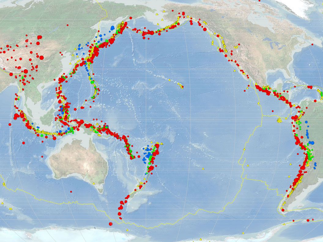
Artificial Intelligence is the key to the future of weather forecasting, a fact well known. But did you know it is also powering earthquake prediction the world over? Yes. Artificial Intelligence techniques like machine learning are gradually being enlisted in forecasting seismic activity.

While earthquake prediction has not yet become an exact science, efforts are on to make improvements and make forecasts reliable. For this, AI powered neural networks, the same technology behind the success of driverless cars and digital assistants, is being used to enhance research based on seismic data.

Neural Networks

A report says that, “Scientists say seismic data is remarkably similar to the audio data that companies like Google and Amazon use in training neural networks to recognize spoken commands on coffee-table digital assistants like Alexa.”

When it comes to studying earthquakes, it is the computer, a fast and able machine, looking for patterns in mountains of data rather than relying on the weary eyes of a scientist. Also, instead of a sequence of words, what the computer is studying is a sequence of ground-motion measurements.

Studying Aftershocks
Image Source: cbs8.com

Studying Aftershocks

Scientists in the US have experimented with neural networks to accelerate earthquake analysis and the speed at which they were producing results and studies was 500 times faster than they could in the past. Also, AI is not only useful in studying earthquakes but it is being used in forecasting earthquake aftershocks as well.

In fact, researchers say it is a time of great scientific advancement, so much so, that “technology can do as well as — or better than — human experts”.

Artificial Intelligence
Image Source: smithsonianmag.com

Artificial Intelligence

Geophysicist Paul Johnson’s team in the US has been studying earthquakes for quite some time now and it has made advancements in “using pattern-finding algorithms similar to those behind recent advances in image and speech recognition and other forms of artificial intelligence, (where) he and his collaborators successfully predicted temblors in a model laboratory system — a feat that has since been duplicated by researchers in Europe”, says a report.

Now Mr Johnson’s team has published a paper wherein artificial intelligence has been used to study slow slip earthquakes in the Pacific Northwest. While advancements are being made in the field of studying slow slip earthquakes, it is the bigger and more potent ones that really need to be studied. But they are rare. So the question remains – Will Machine Learning be able to analyse a small data set and predict with confidence the next big earthquake?

Data Science Machine Learning Certification

Machine Learning 

Researchers claim “that their (machine learning) algorithms won’t actually need to train on catastrophic earthquakes to predict them.” Studies conducted recently suggest “seismic patterns before small earthquakes are statistically similar to those of their larger counterparts”. So, a computer trained on hundreds and thousands of those small temblors might be able enough to predict the big ones.

For more on artificial intelligence, and its varied applications, do peruse the DexLab Analytics website today. DexLab Analytics is a premier institute in India offering Machine Learning courses in Delhi.


.

ROC-Curve-New-Plotting-API-Release Highlights for Scikit-learn 0.22

ROC-Curve-New-Plotting-API-Release Highlights for Scikit-learn 0.22

Today we are going to learn about the new releases from Scikit-learn version 0.22, a machine learning library in Python. We, through this video tutorial, aim to learn about the much talked about new release called Plotting API. Prior to this version, Scikit-learn did not have a function to plot the ROC curve.

A new plotting API is available for creating visualizations. The new API allows for quickly adjusting the visuals of a plot without involving any recomputation. It is also possible to add different plots to the same figure. In this tutorial we are going to study the plotting of the ROC curve.

The code sheet is provided in a Github repository here.


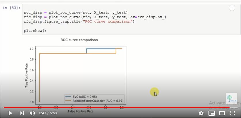
We will attempt to plot the ROC curve on two different algorithms and compare which one is a better function. First we choose to make a classification data. Then we go on to plot the ROC curve using SVC classifier and then further plot the curve using a random forest classifier.

Fig. 1

Fig. 1

For more on this do watch the video attached herewith. This tutorial was brought to you by DexLab Analytics. DexLab Analytics is a premiere Machine Learning institute in Gurgaon.


.

How Machine Learning Helped Demystify Locust Breeding Sites

How Machine Learning Helped Demystify Locust Breeding Sites

Even as the coronavirus pandemic rages on and India is living through a strict lockdown to abate the spread of the novel virus, a disastrous spell of a plague of crop destroying locusts has struck Rajasthan, Gujarat and parts of Madhya Pradesh.

Threatening to balloon into an agrarian crisis, the destruction of crops on this scale is being seen as one “worst in decades”. In fact, such large scale breeding of locusts and an attack by them is the worst in 27 years, government officials said.

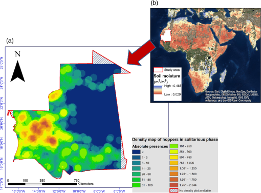
In such frightening circumstances, what we can truly bank upon to detect and fight locust attacks is advanced technology like machine learning techniques. This essay aims to demystify how machine learning can be used to detect locust breeding patterns by studying soil moisture through remote sensing.

The Study

Image Source: spiedigitallibrary.org

A study called “Machine learning approach to locate desert locust breeding areas based on ESA CCI soil moisture” shows how researchers have “used two machine learning algorithms (generalized linear model and random forest) to evaluate the link between hopper presences and SM (Soil Moisture) conditions under different time scenarios…It was found that an area becomes suitable for breeding when the minimum SM values are over 0.07  m3  /  m3 during 6 days or more. These results demonstrate the possibility to identify breeding areas in Mauritania by means of SM, and the suitability of ESA (European Space Agency) CCI (Climate Change Initiative) SM product to complement or substitute current monitoring techniques based on precipitation datasets.”

The Findings

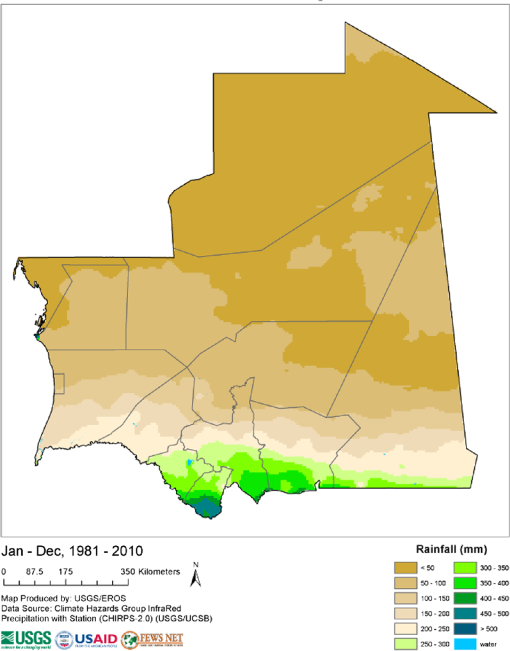
The study found that “it is widely assumed” that rainfall over 25 mm in two consecutive months is conducive to locust breeding. Likewise, various soil moisture conditions affect breeding patterns greatly. So, the study finds that it is important to have “variable creation as a previous step to modeling”. Different time intervals of locust breeding were tested by the researchers for model creation. Also, different soil moisture values were considered.

Image Source: spiedigitallibrary.org

It was found that the “highest performance was acquired by the RF (Random Forest) algorithm when dividing the whole survey time into ranges of 6 days, and selecting the minimum SM as the variable value.” GLMs of Generalised Linear Models, however, did not work well according to the study.

The applied methodology of machine learning offers promising results to accurately identify breeding areas based on data pertaining to 30 years of SM values. The ESA CCI soil moisture data is one of the most authoritative ones in the world. Thus the researchers who conducted this study are confident that their results signify a breakthrough in locust monitoring technique prevalence in the world.

Data Science Machine Learning Certification

Conclusion

This study, thus, proposes a machine learning approach based on SM time series “to predict breeding areas, by means of remote sensing”. Artificial Intelligence and Machine Learning will help future researchers and scientists to study and produce better warning systems based on the results of this study. In this study only soil moisture data has been used but more variables like temperatures can also be taken into account to accurately predict breeding grounds in the future.

For more on machine learning applications, do peruse the Dexlab Analytics website today. This article was brought to you by DexLab Analytics, a premier institute offering Machine Learning courses in Delhi.


The blog has been sourced fromMachine learning approach to locate desert locust breeding areas based on ESA CCI soil moisture


.

Call us to know more