Machine Learning Certification Courses Archives - DexLab Analytics | Big Data Hadoop SAS R Analytics Predictive Modeling & Excel VBA

Time Series Analysis & Modelling with Python (Part II) – Data Smoothing

Posted on January 20, 2021January 20, 2021 by Dexlab

Data Smoothing is done to better understand the hidden patterns in the data. In the non- stationary processes, it is very hard to forecast the data as the variance over a period of time changes, therefore data smoothing techniques are used to smooth out the irregular roughness to see a clearer signal.

In this segment we will be discussing two of the most important data smoothing techniques :-

Moving average smoothing
Exponential smoothing

Moving average smoothing

Moving average is a technique where subsets of original data are created and then average of each subset is taken to smooth out the data and find the value in between each subset which better helps to see the trend over a period of time.

Lets take an example to better understand the problem.

Suppose that we have a data of price observed over a period of time and it is a non-stationary data so that the tend is hard to recognize.

QTR (quarter)	Price
1	10
2	11
3	18
4	14
5	15
6	?

In the above data we don’t know the value of the 6^th quarter.

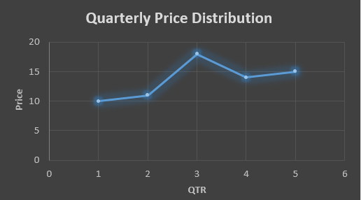
….fig (1)

The plot above shows that there is no trend the data is following so to better understand the pattern we calculate the moving average over three quarter at a time so that we get in between values as well as we get the missing value of the 6^th quarter.

To find the missing value of 6^th quarter we will use previous three quarter’s data i.e.

MAS = = 15.7

QTR (quarter)	Price
1	10
2	11
3	18
4	14
5	15
6	15.7

MAS = = 13

MAS = = 14.33

QTR (quarter)	Price	MAS (Price)
1	10	10
2	11	11
3	18	18
4	14	13
5	15	14.33
6	15.7	15.7

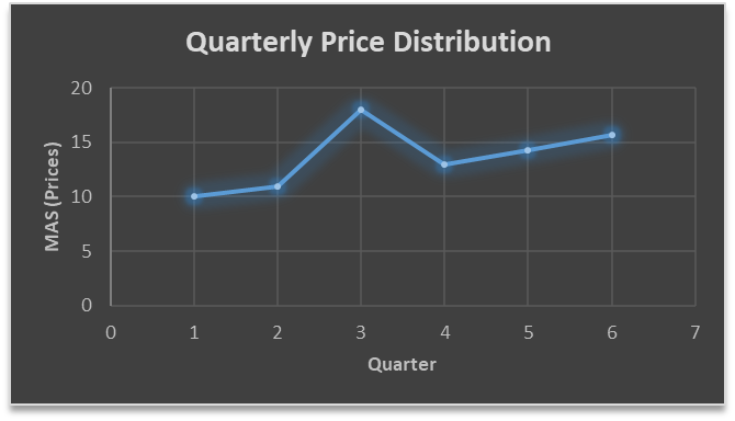
….. fig (2)

In the above graph we can see that after 3^rd quarter there is an upward sloping trend in the data.

Exponential Data Smoothing

In this method a larger weight ( ) which lies between 0 & 1 is given to the most recent observations and as the observation grows more distant the weight decreases exponentially.

The weights are decided on the basis how the data is, in case the data has low movement then we will choose the value of closer to 0 and in case the data has a lot more randomness then in that case we would like to choose the value of closer to 1.

EMA= F_t= F_t-1 + (A_t-1 – F_t-1)

Now lets see a practical example.

For this example we will be taking = 0.5

Taking the same data……

QTR (quarter)	Price (A_t)	EMS Price(F_t)
1	10	10
2	11	?
3	18	?
4	14	?
5	15	?
6	?	?

To find the value of yellow cell we need to find out the value of all the blue cells and since we do not have the initial value of F₁ we will use the value of A_1.Now lets do the calculation:-

F₂=10+0.5(10 – 10) = 10

F₃=10+0.5(11 – 10) = 10.5

F₄=10.5+0.5(18 – 10.5) = 14.25

F₅=14.25+0.5(14 – 14.25) = 14.13

F₆=14.13+0.5(15 – 14.13)= 14.56

QTR (quarter)	Price (A_t)	EMS Price(F_t)
1	10	10
2	11	10
3	18	10.5
4	14	14.25
5	15	14.13
6	14.56	14.56

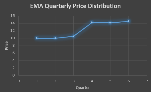
In the above graph we see that there is a trend now where the data is moving in the upward direction.

So, with that we come to the end of the discussion on the Data smoothing method. Hopefully it helped you understand the topic, for more information you can also watch the video tutorial attached down this blog. The blog is designed and prepared by Niharika Rai, Analytics Consultant, DexLab Analytics DexLab Analytics offers machine learning courses in Gurgaon. To keep on learning more, follow DexLab Analytics blog.

The Evolution of Neural Networks

Posted on July 25, 2017November 24, 2018 by Dexlab

The Evolution of Neural Networks

Recently, Deep Learning has gone up from just being a niche field to mainstream. Over time, its popularity has skyrocketed; it has established its position in conquering Go, learning autonomous driving, diagnosing skin cancer, autism and becoming a master art forger.

Before delving into the nuances of neural networks, it is important to learn the story of its evolution, how it came into limelight and got re-branded as Deep Learning.

The Timeline:

Warren S. McCulloch and Walter Pitts (1943): “A Logical Calculus of the Ideas Immanent in Nervous Activity”

Here, in this paper, McCulloch (neuroscientist) and Pitts (logician) tried to infer the mechanisms of the brain, producing extremely complicated patterns using numerous interconnected basic brain cells (neurons). Accordingly, they developed a computer-programmed neural model, known as McCulloch and Pitt’s model of a neuron (MCP), based on mathematics and algorithms called threshold logic.

Marvin Minsky (1952) in his technical report: “A Neural-Analogue Calculator Based upon a Probability Model of Reinforcement”

Being a graduate student at Harvard University Psychological Laboratories, Minsky executed the SNARC (Stochastic Neural Analog Reinforcement Calculator). It is possibly the first artificial self-learning machine (artificial neural network), and probably the first in the field of Artificial Intelligence.

Marvin Minsky & Seymour Papert (1969): “Perceptron’s – An Introduction to Computational Geometry” (seminal book):

In this research paper, the highlight has been the elucidation of the boundaries of a Perceptron. It is believed to have helped usher into the AI Winters – a time period of hype for AI, in which funds and publications got frozen.

Kunihiko Fukushima (1980) – “Neocognitron: A Self-organizing Neural Network Model for a Mechanism of Pattern Recognition Unaffected by Shift in Position” (this concept is an important component for Convolutional Neural Network – LeNet)

Fukushima conceptualized a whole new, much improved neural network model, known as ‘Neocognitron’. This name is derived from ‘Cognitron’, which is a self-organizing multi layered neural network model proposed by [Fukushima 1975].

David B. Parker (April 1985 & October 1985) in his technical report and invention report – “Learning – Logic”

David B. Parker reinvented Backpropagation, by giving it a new name ‘Learning Logic’. He even reported it in his technical report as well as filed an invention report.

Yann Le Cun (1988) – “A Theoretical Framework for Back-Propagation”

You can derive back-propagation through numerous ways; the simplest way is explained in Rumelhart et al. 1986. On the other hand, in Yann Le Cun 1986, you will find an alternative deviation, which mainly uses local criteria to be minimized locally.

J.S. Denker, W.R. Garner, H.P. Graf, D. Henderson, R.E. Howard, W. Hubbard, L.D. Jackel, H.S. Baird, and I. Guyon at AT&T Bell Laboratories (1989): “Neural Network Recognizer for Hand-Written ZIP Code Digits”

In this paper, you will find how a system ascertains hand-printed digits, through a combination of neural-net methods and traditional techniques. The recognition of handwritten digits is of crucial notability and of immense theoretical interest. Though the job was comparatively complicated, the results obtained are on the positive side.

Yann Le Cun, B. Boser, J.S. Denker, D. Henderson, R.E. Howard, W. Hubbard, L.D. Jackel at AT&T Bell Laboratories (1989): “Backpropagation Applied to Handwritten ZIP Code Recognition”

A very important real-world application of backpropagation (handwritten digit recognition) has been addressed in this report. Significantly, it took into account the practical need for a chief modification of neural nets to enhance modern deep learning.

Besides Deep Learning, there are other kinds of architectures, like Deep Belief Networks, Recurrent Neural Networks and Generative Adversarial Networks etc., which can be discussed later.

For comprehensive Machine Learning training Gurgaon, reach us at DexLab Analytics. We are a pioneering data science online training platform in India, bringing advanced machine learning courses to the masses.

Interested in a career in Data Analyst?
To learn more about Data Analyst with Advanced excel course – Enrol Now.
To learn more about Data Analyst with R Course – Enrol Now.
To learn more about Big Data Course – Enrol Now.
To learn more about Machine Learning Using Python and Spark – Enrol Now.
To learn more about Data Analyst with SAS Course – Enrol Now.
To learn more about Data Analyst with Apache Spark Course – Enrol Now.
To learn more about Data Analyst with Market Risk Analytics and Modelling Course – Enrol Now.

Call us to know more

Gurgaon

Kolkata