Tag: data visualization with Python

In our fifth installment of the visualization series using Python programming language, we introduce you to another powerful library in Python that is the Pandas_bokeh library. So, let’s find out what you can achieve with Pandas_bokeh library.

Pandas_bokeh is a library which can help you create interactive graphs in python. One can zoom in, zoom out, select a certain portion of the graph to see, move the plot left, right and center, create tabs in case they want to see a single plot at a time, create multiple plots at a time, create widgets like dropdown list, check boxes, radio buttons, slider etc. It is similar to the shiny app which is used in the r programming language  but simpler and faster.

How to install pandas_bokeh?

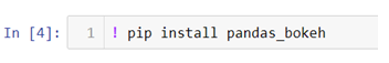
In the above code we are changing our jupyter notebook code cell into a command line by using ! and then we can use pip (python installation package) to install the library.

How to create a simple line plot using pandas_bokeh ?

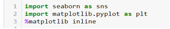
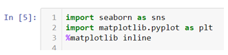
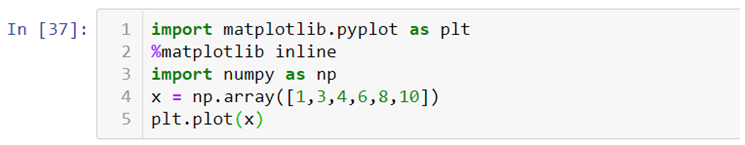
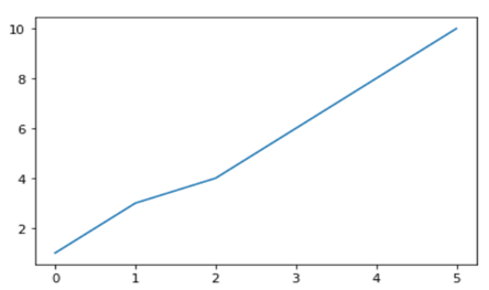
The first thing to do is import the libraries which we will be using to create a line plot.

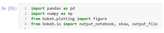
• We will be creating our own dataset here and for that we need to import Numpy and Pandas libraries. Also we will be importing .figure() method from plotting module to create our canvas on which we will be building our graph from the scratch and we will also be importing .output_notebook() method to visualize our graph on jupyter notebook and to visualize our graph on a new tab and save at the same time we can use .output_file() method.
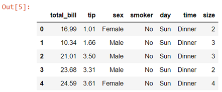
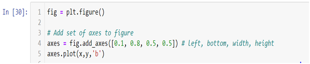
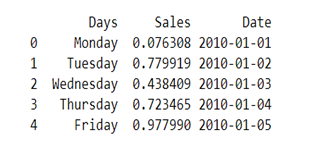
• The Dataset we are creating here will have three columns ‘Days’, ‘Sales’ and ‘Date’.
  
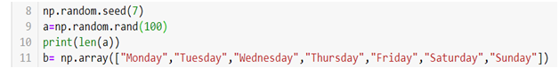
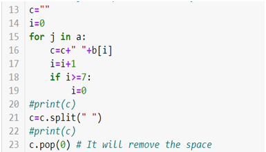
• We will be creating a dataset with hundred observations in each column so for that we are using .rand() method to generate hundred random numbers and that will be our ‘Sales’ column data. Now for our ‘Days’ column we will be creating a loop which will run hundred times and each time an array index value will be saved in a variable c which has an empty string and .split() method is then used to create a list of that string.
• For creating a ‘Date’ column we will be using the following code
  
  
• At last create a data frame we will be using .DataFrame() method.
  
  
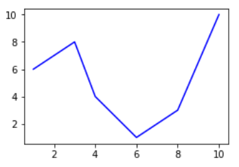
• Now to create two line graphs on a single canvas we will be using object-oriented programming.
  
  
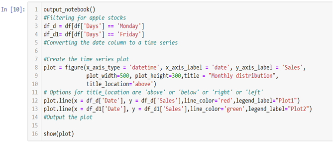
• To build the graph on the jupyter notebook we are using .output_notebook() method and in case you want to plot the graph on a new tab you can use .output_file(“filename.html”) method.

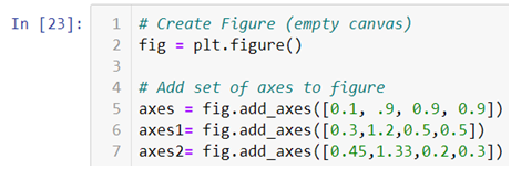
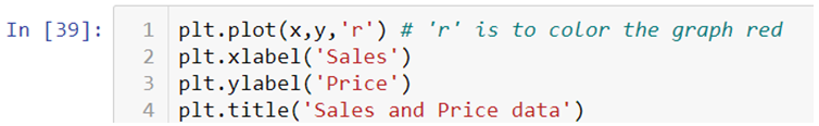
In the above line of codes we are creating two separate data frames df_d and df_d1 each containing Monday and Friday’s sales and dates separately now all we need to do is build a canvas using .figure() method and use few other arguments like x_axis_type to define the data type of the x axis and x_axis_label and y_axis_label to set graph labels, to adjust width and height of the canvas we have used plot_width and plot_height argument and to set title and title location we have used title and title_location. Once we have our canvas ready we can use .line() method and add x axis and y axis data to plot our graphs.

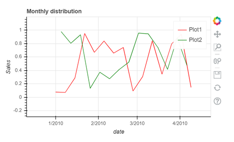
• To interact with your graph you can use the icons on the right hand side corner which will help you zoom in and out, look at a certain part of the graph, scroll to zoom in and out, save your plot and reset the changes made by you using the side icons.

The video tutorial attached below will help you gain better understanding. 

At the end of this segment you must have become familiar with the nuances of the Pandas_bokeh library. As you continue on with the series, you will realize that you are becoming an expert in visualization. On Dexlab Analytics blog, you will find interesting blogs on various topics related to Python certification training.

This is the 4th part of the series on visualization using Python programming language, where we will continue our discussion on the Seaborn library. Now that you have become familiar with the basics of the Seaborn library, you will be learning specific skills such as learning to create a box plot using Seaborn. So, let’s begin.

Seaborn library offers a list of pre-defined methods to create semi-flexible plots in Python and one of them is. boxplot() method. But what is a box plot?

Answer:- A box plot often known as box and whisker plot is a graph created to visualize the distribution of numerical data and skewness through displaying the data quartiles (or percentiles) and median.

Creating a box plot

Let’s begin by importing the Seaborn and Matplotlib library.

We will again be using the tips dataset which is a pre-defined dataset in Seaborn

Data description:- This is a dataset of a restaurant which keeps a record of the amount of bill paid by a customer, tip amount over the total bill paid, gender of the customer, whether he or she was a smoker or not, the day on which they ate at the restaurant, what was the time when they ate at the restaurant and the size of the table they booked.

To create a box plot we will be using .boxplot() method.

On the x axis we have day column having categorical data type and on the y axis we have total_bill column having numerical data type. Thus for each day with the help of a box plot we will  be able to visualize how the total_bill changes around its median value.

To add title to the graph we can use. title() method from the Matplotlib library

To add color to your graph you can use palette argument

We are adding a list of palette colors in this blog down below:-

You can replace the color mentioned in the above code to see which color variations you would prefer in your graph. For example

Here we are using color palette ‘CMRmap’ to change my graph color from different shades of blues to a completely different color range i.e. from blues to orange, violet, pale yellow etc.

This tutorial hopefully, has clarified the concept and you can now create boxplots with Seaborn. Since this is a series you need to keep track of all the parts to be a visualization expert as we take you through the process step by step. Follow the Dexlab Analytics blog to access more informative posts on different topics including python for data analysis.

Go through the video tutorial attached below to get more in-depth knowledge.

Classroom or Online Certification Courses to get you started

To learn more about Data Analyst with Advanced excel course – Enrol NowTo learn more about Big Data Course – Enrol Now
To learn more about Machine Learning Using Python and Spark – Enrol NowTo learn more about Data Analyst with SAS Course – Enrol Now.
To learn more about Data Analyst with Apache Spark Course – Enrol Now
To learn more about Data Analyst with Market Risk Analytics and Modelling Course – Enrol Now 

In the last blog that covered Part 1 of the visualization series using Python programming language, we have learned the basics of the Matplotlib Library. Now that our grasp on the basics is strong we would move further. Let’s break it all down with a more formal introduction of Matplotlib’s Object Oriented API. This means we will instantiate figure objects and then call methods or attributes from that object.

Introduction to the Object Oriented Method

The main idea in using the more formal Object Oriented method is to create figure objects and then just call methods or attributes off of that object. This approach is nicer when dealing with a canvas that has multiple plots on it.

How to make multiple plots using .add_axes()

To begin, we create a figure instance. Then we can add axes to that figure where .figure()is a method which helps us create an empty canvas and then we use .add_axes() method to give the position where the plot is to be made. The positional arguments [left, bottom, width, height] help us decide from where the graph should begin within the canvas and what should be the width and the height of the graph. Since the area of the graph is 100% (1.0), the range of the positional argument should be between 0 and 1 and in case you want to plot the graph half within and half outside the canvas, you can go beyond the specified range depending upon your needs.

Let’s  quickly get to the coding part now.

• In the above line of codes we are simply importing the Matplotlib library and creating a data which we want to plot.

• plt.figure()method is helping us create an empty canvas and then we are giving the positional values to the .add_axes() method. As you can see we are using a variable named fig to save our canvas and then using the same variable as an object to add an axes to the canvas. Now all we need to do is use that axes to build are graph by adding x and y data.
  
• Now you must be wondering why we aren’t able to see a plot in the corner of the canvas? It is because this procedure works only if we were to build multiple plots. So now let’s see how we can use the .add_axes() method to build multiple plots on top of each other.

• In the above line of codes we are creating three axes and each axes is smaller than the other so that we are able to plot multiple graphs on top of each other.

• Here we are making three different graphs and each graph has its own title and x axis and y axis labels. But to add title and axis labels we are now using .set_title(), .set_xlabel(), and .set_ylabel() instead of .title(), .xlabel() and .ylabel(). In axes2.plot() we are also using RGB color instead of using the predefined color in .plot() method. You can use your favorite color too by simply typing RGB color picker in your Google search and copy pasting the color code in the .plot() method. After running the above code we get the following graph:-
  

How to make multiple plots using .subplots()

.subplots() method is similar to the previous .subplot() method, the only difference is that now we use it on a canvas.

• In the .subplots() we do not mention the plot number instead we use plot indexing method to build graph.
  
  
• As you can see we are accessing the index number to build our plot and then using .tight_layout() method to keep the graphs from overlapping. After running the above code we get the following graphs:-

Do not forget to check out the video tutorial attached below to learn how this method works. Keep following the series to upgrade your skills and to explore more informative posts on topics like Python Programming training you need to follow the Dexlab Analytics blog.

Classroom or Online Certification Courses to get you started

To learn more about Data Analyst with Advanced excel course – Enrol NowTo learn more about Big Data Course – Enrol Now
To learn more about Machine Learning Using Python and Spark – Enrol NowTo learn more about Data Analyst with SAS Course – Enrol Now.
To learn more about Data Analyst with Apache Spark Course – Enrol Now
To learn more about Data Analyst with Market Risk Analytics and Modelling Course – Enrol Now