Data Science training Archives - DexLab Analytics | Big Data Hadoop SAS R Analytics Predictive Modeling & Excel VBA

Time Series Analysis Part I

Posted on January 18, 2021January 18, 2021 by Dexlab

A time series is a sequence of numerical data in which each item is associated with a particular instant in time. Many sets of data appear as time series: a monthly sequence of the quantity of goods shipped from a factory, a weekly series of the number of road accidents, daily rainfall amounts, hourly observations made on the yield of a chemical process, and so on. Examples of time series abound in such fields as economics, business, engineering, the natural sciences (especially geophysics and meteorology), and the social sciences.

Univariate time series analysis- When we have a single sequence of data observed over time then it is called univariate time series analysis.
Multivariate time series analysis – When we have several sets of data for the same sequence of time periods to observe then it is called multivariate time series analysis.

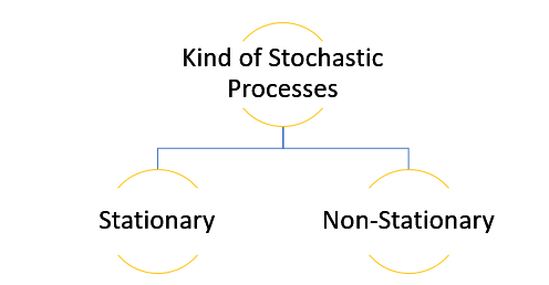
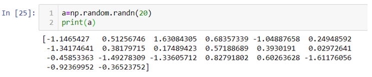
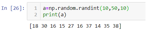
The data used in time series analysis is a random variable (Yt) where t is denoted as time and such a collection of random variables ordered in time is called random or stochastic process.

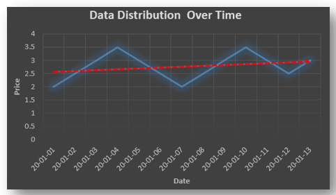
Stationary: A time series is said to be stationary when all the moments of its probability distribution i.e. mean, variance , covariance etc. are invariant over time. It becomes quite easy forecast data in this kind of situation as the hidden patterns are recognizable which make predictions easy.

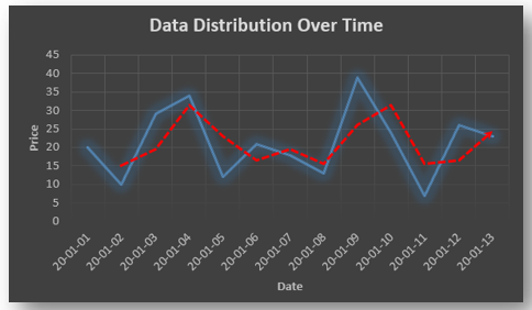
Non-stationary: A non-stationary time series will have a time varying mean or time varying variance or both, which makes it impossible to generalize the time series over other time periods.

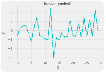
Non stationary processes can further be explained with the help of a term called Random walk models. This term or theory usually is used in stock market which assumes that stock prices are independent of each other over time. Now there are two types of random walks:
Random walk with drift : When the observation that is to be predicted at a time ‘t’ is equal to last period’s value plus a constant or a drift (α) and the residual term (ε). It can be written as
Yt= α + Yt-1 + εt
The equation shows that Yt drifts upwards or downwards depending upon α being positive or negative and the mean and the variance also increases over time.
Random walk without drift: The random walk without a drift model observes that the values to be predicted at time ‘t’ is equal to last past period’s value plus a random shock.
Yt= Yt-1 + εt
Consider that the effect in one unit shock then the process started at some time 0 with a value of Y0
When t=1
Y1= Y0 + ε1
When t=2
Y2= Y1+ ε2= Y0 + ε1+ ε2
In general,
Yt= Y0+∑ εt
In this case as t increases the variance increases indefinitely whereas the mean value of Y is equal to its initial or starting value. Therefore the random walk model without drift is a non-stationary process.

So, with that we come to the end of the discussion on the Time Series. Hopefully it helped you understand time Series, for more information you can also watch the video tutorial attached down this blog. DexLab Analytics offers machine learning courses in delhi. To keep on learning more, follow DexLab Analytics blog.

Theory of Estimation Part-I: The Introduction

Posted on November 27, 2020November 27, 2020 by Dexlab

The theory of estimation is a branch in statistics that provides numerical values of the unknown parameters of the population on the basis of the measured empirical data that has a random component. This is a process of guessing the underlying properties of the population by observing the sample that has been taken from the population. The idea behind this is to calculate and find out the approximate values of the population parameter on the basis of a sample statistics.

Population:- All the items in any field of inquiry constitutes to a “Population”. For example all the employees of a factory is a population of that factory and the population mean is represented and the size of the population is represented by N.

Sample:- Selection of few items from the population constitutes to a sample and the mean of the sample is represented by and the sample size is represented by n

Statistics:- Any statistical measure calculated on the basis of sample observations is called Statistic. Like sample mean, sample standard deviation, etc.

Estimator:- In general estimator acts as a rule, a measure computed on the basis of the sample which tells us how to calculate the values of the estimate. It is a functional form of all sample observations prorating a representative value of the collected sample.

Suppose we have a random sample x_1,x_2,…,x_n on a variable x, whose distribution in the population involves an unknown parameter. It is required to find an estimate of on the basis of sample values.

Unbiasedness:-A statistic t is said to be an unbiased estimator if E(β ̂)= βi.e. observed value is equal to the expected value. In case E(β ̂)≠ β then the estimator is biased estimator.

Consistency:- One of the most desirable property of good estimator is that its accuracy should increase when the sample becomes larger i.e. the error between the expected value and the observed value reduces as the size of the sample increases E(β ̂ )- β=0

Efficiency:-An estimator is said to be an efficient estimator if it has the smallest variance compared to all the consistent and unbiased estimators. If consistent estimator exists whose sampling variance is less than that of any other consistent estimator, it is said to be “most efficient”; and it provides a standard for the measurement of ‘efficiency’ of a statistic.

Sufficiency:- An estimator is said to be sufficient if it contains all information in the sample about .

At the end of this discussion, hopefully, you have learned what theory of estimation is. Watch the video tutorial attached below to learn more about this. DexLab Analytics is a data science training institute in gurgaon, that offers advanced courses. Follow the blog section to access more informative posts like this.

An Introductory Guide to NumPy

Posted on November 25, 2020November 25, 2020 by Dexlab

NumPy also known as numerical python, is a library consisting of multidimensional array objects and a collection of routines for processing those arrays. Using NumPy, mathematical and logical operations on arrays can be performed without it which was not possible. For example-

Multiplication of two lists will cause an error as a data structure like lists, tuple, dictionaries and sets do not allow mathematical operations.

Therefore we need NumPy to covert our data structures like lists into 1d, 2d, 3d or nd arrays so that mathematical operations can be performed. U

We can use .array() methods to create these arrays.

Now let’s check out few examples and also perform few mathematical operations to have a better understanding.

In the above code we first import NumPy library and then use .array() method to two 1d-array a1 and b1 using the list we previously created.
Now let’s multiply a1 and b1 array.
Now let’s use .array() method to directly create an array.

Arrays can be created using lists, tuples and dictionaries as you can see in the above example.

Now for 2-d arrays recall that we can also make list of lists. Let’s use that to create 2d-arrays.

2d-arrays can also be created using tuples.

Remember that we are not using these as matrices because matrix multiplication is an entirely different thing we are just trying to perform mathematical operations which were otherwise not possible.

Random Module

Numpy also has various ways with which we can create array of random numbers which then can be used in number of ways like generating a data for practice purposes or for building beautiful graphs for a presentation.

Given below is a list of type of random numbers you can generate

.rand() :- This particular method helps you generate uniformly distributed random numbers i.e. numbers between 0 and 1 where each number between 0 and 1 will have equal probability to be in the sample dataset.

The above code generates a 2d-array with values between 0 and 1.

.randn():- This method generates normally distributed random numbers i.e. numbers between -3 and +3 where mean=median=mode and ploted gives a bell shaped curve.

Here the 20 random numbers are generated ranging between -3 and + 3.

Note:- Remember that the data is randomly picked from the normally distributed values between -3 and +3 so the graph is not bell shaped but the original data from which the values are being picked randomly is bell shaped with mean=median-mode.

.randint():-This method generates random integers between a given range.

So, with that we come to the end of the discussion on the Numpy. Hopefully it helped you understand Numpy, for more information you can also watch the video tutorial attached down this blog. DexLab Analytics offers machine learning courses in delhi. To keep on learning more, follow DexLab Analytics blog.

Linear Regression Part II: Predictive Data Analysis Using Linear Regression

Posted on November 23, 2020November 23, 2020 by Dexlab

In our previous blog we studied about the basic concepts of Linear Regression and its assumptions and let’s practically try to understand how it works.

Given below is a dataset for which we will try to generate a linear function i.e.

y=b₀+b₁Xi

Where,

y= Dependent variable

Xi= Independent variable

b₀ = Intercept (coefficient)

b₁= Slope (coefficient)

To find out beta (b₀& b₁) coefficients we use the following formula:-

Let’s start the calculation stepwise.

First let’s find the mean of x and y and then find out the difference between the mean values and the X_i and Y_ie. (x-x ̅ ) and (y-y ̅ ).
Now calculate the value of (x-x ̅ )² and (y-y ̅ )². The variation is squared to remove the negative signs otherwise the summation of the column will be 0.
Next we need to see how income and consumption simultaneously variate i.e. (x-x ̅ )* (y-y ̅ )

Now all there is left is to use the above calculated values in the formula:-

As we have the value of beta coefficients we will be able to find the y ̂(dependent variable) value.

We need to now find the difference between the predicted y ̂ and observed y which is also called the error term or the error.

To remove the negative sign lets square the residual.

What is R²and adjusted R² ?

R² also known as goodness of fit is the ratio of the difference between observed y and predicted and the observed y and the mean value of y.

Hopefully, now you have understood how to solve a Linear Regression problem and would apply what you have learned in this blog. You can also follow the video tutorial attached down the blog. You can expect more such informative posts if you keep on following the DexLab Analytics blog. DexLab Analytics provides data Science certification courses in gurgaon.

ANOVA Part-II: What is Two-way ANOVA?

Posted on November 18, 2020November 18, 2020 by Dexlab

In my previous blog, I have already introduced you to a statistical term called ANOVA and I have also explained you what one-way ANOVA is? Now in this particular blog I will explain the meaning of two-way ANOVA.

The below image shows few tests to check the relationship/variation among variables or samples. When it comes to research analysis the first thing that we should do is to understand the sample which we have and then try to disintegrate the dataset to form and understand the relationship between two or more variables to derive some kind of conclusion. Once the relation has been established, our job is to test that relationship between variables so that we have a solid evidence for or against them. In case we have to check for variation among different samples, for example if the quality of seed is affecting the productivity we have to test if it is happening by chance or because of some reason. Under these kind of situations one-way ANOVA comes in handy (analysis on the basis of a single factor).

Two-way ANOVA

Two-way ANOVA is used when we are testing the variations among samples on the basis two factors. For example testing variation on the basis of seed quality and fertilizer.

Hopefully you have understood what Two-way ANOVA is. If you need more information, check out the video tutorial attached down the blog. Keep on following the DexLab Analytics blog, to find more information about Data Science, Artificial Intelligence. DexLab Analytics offers data Science certification courses in gurgaon.

An Introduction to Sampling and its Types

Posted on November 16, 2020November 16, 2020 by Dexlab

Sampling is a technique in which a predefined number of observation is taken from a large population for the purpose of statistical analysis and research.

There are two types of sampling techniques:-

Random Sampling

Random sampling is a sampling technique in which each observation has an equal probability of being chosen. This kind of sample should be an unbiased representation of the population.

Types of random sampling

Simple Random Sampling:- Simple random sampling is a technique in which any observation can be chosen and each observation has an equal probability of being selected.
Stratified Random Sampling:- In this sampling technique we create sub-group of the population with similar attributes and characteristics and then out of those sub-groups we then include each category in our sample with the probability of choosing each observation from the sub-group being equal.
Systematic Sampling:- This is a sampling technique where the first observation is selected randomly and then every kth element is chosen randomly to be included in our sample.
k= 2, here the first observation is selected randomly and after that every second element is included in the sample.
Cluster Sampling:- This is a sampling technique in which the data is grouped into small sub-groups called clusters with random categories and then from those clusters random observation is selected which then is included in the sample.

Two clusters are created from which then random observation will be chosen to form the sample.

Non-Random Sampling :- It is a sampling technique in which an element of biasedness is introduced which means that an observation is selected for the sample on the basis of not probability but choice.

Types of non-random sampling:-

Convenience Sampling:- When a sample observation is drawn from the population based on how comfortable it is for you to take the observation it is called convenience sampling. For example when you have a survey sheet that is to be filled by students from all the departments of your college but you only ask your friends to fill the survey sheet.
Judgment Sampling:– When the sample observation drawn from the population is based on your professional judgment or past experience, it is called judgment sampling.
Quota Sampling:– When you draw a sample observation from the population that is based on some specific attribute, it is called quota sampling. For example, taking sample of people over and above 50 years.
Snow Ball Sampling:– When survey subjects are selected based on referral from other survey respondents, it is called snow ball sampling.

Sampling and Non-sampling errors

Sampling errors:- It occurs when the sample is not representative of the entire population. For example a sample of 10 people with or without COVID-19 cannot tell whether or not the entire population of a country is COVID positive.

Non-sampling error:-This kind of error occurs during data collection. For example, during data collection if you falsely specified a name, it will be considered a non-sampling error.

So, with that this discussion on Sampling wraps up, hopefully, at the end of this you have learned what Sampling is, what are its variations and how do they all work. If you need further clarification, then check out our video tutorial on Sampling attached down the blog. DexLab Analytics provides the best data science course in gurgaon, keep following the blog section to stay updated.

Hypothesis Testing: An Introduction

Posted on November 11, 2020November 11, 2020 by Dexlab

You must be familiar with the phrase hypothesis testing, but, might not have a very clear notion regarding what hypothesis testing is all about. So, basically the term refers to testing a new theory against an old theory. But, you need to delve deeper to gain in-depth knowledge.

Hypothesis are tentative explanations of a principal operating in nature. Hypothesis testing is a statistical method which helps you prove or disapprove a pre-existing theory.

Hypothesis testing can be done to check whether the average salary of all the employees has increased or not based on the previous year’s data, testing can be done to check if the percentage of passengers increased or not in the business class due to introduction of a new service and testing can also be done to check the differences in the productivity varied land.

There are two key concepts in testing of hypothesis:-

Null Hypothesis:- It means the old theory is correct, nothing new is happening, the system is in control, old standard is correct etc. This is the theory you want to check if is true or not. For example if a ice-cream factory owner says that their ice-cream contains 90% milk, this can be written as:-

Alternative Hypothesis:- It means new theory is correct, something is happening, system is out of control, there are new standards etc. This is the theory you check against the null hypothesis. For example you say that ice-cream does not contain 90% milk, this can be written as:-

Two-tailed, right tailed and left tailed test

Two-tailed test:- When the test can take any value greater or less than 90% in the alternative it is called two-tailed test ( H190%) i.e. you do not care if the alternative is more or less all you want to know is if it is equal to 90% or no.

Right tailed test:-When your test can take any value greater than 90% (H1>90%) in the alternative hypothesis it is called right tailed test.

Left tailed test:-When your test can take any value less than 90% (H1<90%) in the alternative hypothesis it is called left tailed test.

Type I error and Type II error

->When we reject the null hypothesis when it is true we are committing type I error. It is also called significance level.

->When we accept the null hypothesis when it is false we are committing type II error.

Steps involved in hypothesis testing

Build a hypothesis.
Collect data
Select significance level i.e. probability of committing type I error
Select testing method i.e. testing of mean, proportion or variance
Based on the significance level find the critical value which is nothing but the value which divides the acceptance region from the rejection region
Based on the hypothesis build a two-tailed or one-tailed (right or left) test graph
Apply the statistical formula
Check if the statistical test falls in the acceptance region or the rejection region and then accept or reject the null hypothesis

Example:- Suppose the average annual salary of the employees in a company in 2018 was 74,914. Now you want to check whether the average salary of the employees has increased or not in 2019. So, a sample of 112 people were taken and it was found out that the average annual salary of the employees in 2019 is 78,795. σ=14.530.

We will apply hypothesis testing of mean when known with 5% of significance level.

The test result shows that 2.75 falls beyond the critical value of 1.9 we reject the null hypothesis which basically means that the average salary has increased significantly in 2019 compared to 2018.

So, now that we have reached at the end of the discussion, you must have grasped the fundamentals of hypothesis testing. Check out the video attached below for more information. You can find informative posts on Data Science course, on Dexlab Analytics blog.

Linear Regression Part I: A Comprehensive Guide to Linear Regression

Posted on November 9, 2020November 9, 2020 by Dexlab

Today’s blog explores another vital statistical concept Linear Regression, let’s begin. Linear regression is normally used in statistics for predictive modeling. It tries to model a relationship between two independent (explanatory variable) and dependent (explained variable) variables X and Y by fitting a linear equation (Y=b_o+b₁X+U_i) to an observed data.

Assumptions of linear regression

U_i is a random real variable, where U_iis the difference between the observed dependent variable Y and predicted Y variable.
The mean of U_iin any particular period is zero.
The variance of U_i is constant in each period i.e for all values of X, U_i will show the same dispersion around their mean
The variable U_i has a normal distribution i.e the value of U_i (for each X_i) have a bell shaped symmetrical distribution about their zero mean.
The random terms of different observations are independent i.e the covariance of any U_iwith any other U_j is equal to zero.
U_i is independent of the explanatory variable X.
X_iare a set of fixed values in the hypothesised process of repeated sampling which underlies the linear regression model.
In case there are more than one explanatory variables then they are not perfectly linearly correlated.

Linear Regression equation can be written as:

Where,

is the dependent variable

X is the independent variable.

b₀is the intercept (where the line crosses the vertical y-axis)

b₁is the slope

U_i is the error term (difference between ) also called residual or white noise.

Simple linear regression follows the properties of Ordinary Least Square (OLS) which are as follows:-

Unbiased estimator:- E()=b ie. an estimator is unbiased if its bias is 0; E() – b = 0
Minimum Variance:- An estimate is best when it has the smallest variance as compared to any other estimate obtained from other econometric method.
Efficient estimator:- When it has both the previous properties ie.
Linear estimator
Best, Linear, Unbiased estimator (BLUE)
Minimum mean squared error (MSE) estimator:- It is a combination of the unbiasedness and minimum variance properties. An estimator is a minimum MSE estimator if it has the smallest mean square error.

With that the discussion on Linear Regression wraps up here, hopefully it cleared away any confusion you might have and helped you get a grasp on the concept. We have a video discussion on this same topic, which is attached below this blog, check it out for further reference.

Continue to track the DexLab Analytics blog to find informative posts related to Python for data science training.

Why Pursuing a Certification Course in Machine Learning Makes Sense Than Doing Self-Study?

Posted on November 6, 2020November 6, 2020 by Dexlab

If you are aware of the growth opportunities awaiting you in the Machine Learning domain, you must be in a rush to master the Machine Learning skills. Now, there are courses available that aim to sharpen the students with skills they would need to work in a challenging environment. However, some often prefer the self-study mode for developing knowledge in this highly specialized domain. No matter which way you prefer to learn, ultimately your passion and dedication would matter the most, because in both ways you need to put in the hard work and really toil hard to make any progress.

Is self-study a feasible option?

If you have already been through some course and want to go to the advanced level through self-study that’s a different issue, but, for those who are just starting out without any background in science, does it even make any sense to opt for self-study?

Given the way Machine Learning technology is moving fast and creating a demand for professionals with highly specialized industry knowledge, do you think self-study would be enough? Do you think a self-study plan to learn something you have no idea about would work? How much time would you need to devote? What should be your learning route? And how do you know this is the right path to follow?

Before we dive deeper into the discussion, we need to go through some prerequisites for Machine Learning study plan.

Machine learning is a broad field and assuming you are a beginner with no prior knowledge in this domain, you have to be familiar with mathematics, statistics, programming languages, meaning undergoing a Python certification training</strong>, must be proficient in data handling including analysis and modeling, you have to work on algorithms. So, can you pick up all of these skills one by one via self-study? Add to the list the latest Machine Learning tools and applications you need to grasp.

There will be help available in the form of:

There would be vast resources, in forms of e-books, lectures, video tutorials, most of these are free and easily accessible.

There are forums, groups out there which you can join and access help

You can take part in online competitions

Think it through. How long will it take for you to get from one stage to the next?

Even though there being no dearth of resources available you would be struggling with your progress and most importantly you would struggle to keep up with the pace the technology is moving ahead. Picking up a programming language, grasping and mastering concepts of linear algebra, probability, data is going to be a mammoth task.

What difference a certification course can make?

To begin with these courses are designed for people coming from different backgrounds, so, you having or, not having any prior knowledge in mathematics, statistics wouldn’t matter as you would be taught everything from scratch be it math or, Machine Learning Using Python.

The programs are designed for both working professionals as well as for beginners, all you need to do is choose the one that suits your specific level.

These courses are designed to transform you into an industry-ready professional and you would be under the guidance of professionals who are more than familiar with the nuances of the way the industry functions.

The modules would follow a strict schedule and your training path would be well planned out covering all the areas you need to master.

You would learn via hands-on training and get to handle projects. Nothing makes you skilled like hands-on training.

Your journey towards a smarter future needs to be through a well mapped-out path, so, be smart about it. DexLab Analytics offers industry-ready courses on Data Science, Machine Learning course in Gurgaon and AI with Python. Take advantage of the courses that are taught by instructors who have both expertise and experience. Time is indeed money, so, stop wasting time and get down to learning.

Call us to know more

Gurgaon

+91 8676079880

Kolkata

+91 9903662244

×