credit risk analysis training in Bangalore Archives - DexLab Analytics | Big Data Hadoop SAS R Analytics Predictive Modeling & Excel VBA

MongoDB Basics Part-II

Posted on February 20, 2021 by Dexlab

In our previous blog we discussed about few of the basic functions of MQL like .find() , .count() , .pretty() etc. and in this blog we will continue to do the same. At the end of the blog there is a quiz for you to solve, feel free to test your knowledge and wisdom you have gained so far.

Given below is the list of functions that can be used for data wrangling:-

updateOne() :- This function is used to change the current value of a field in a single document.

After changing the database to “sample_geospatial” we want to see what the document looks like? So for that we will use .findOne() function.

Now lets update the field value of “recrd” from ‘ ’ to “abc” where the “feature_type” is ‘Wrecks-Visible’.

Now within the .updateOne() funtion any thing in the first part of { } is the condition on the basis of which we want to update the given document and the second part is the changes which we want to make. Here we are saying that set the value as “abc” in the “recrd” field . In case you wanted to increase the value by a certain number ( assuming that the value is integer or float) you can use “$inc” instead.

2. updateMany() :- This function updates many documents at once based on the condition provided.

3. deleteOne() & deleteMany() :- These functions are used to delete one or many documents based on the given condition or field.

4. Logical Operators :-

“$and” : It is used to match all the conditions.

“$or” : It is used to match any of the conditions.

The first code matches both the conditions i.e. name should be “Wetpaint” and “category_code” should be “web”, whereas the second code matches any one of the conditions i.e. either name should be “Wetpaint” or “Facebook”. Try these codes and see the difference by yourself.

So, with that we come to the end of the discussion on the MongoDB Basics. Hopefully it helped you understand the topic, for more information you can also watch the video tutorial attached down this blog. The blog is designed and prepared by Niharika Rai, Analytics Consultant, DexLab Analytics DexLab Analytics offers machine learning courses in Gurgaon. To keep on learning more, follow DexLab Analytics blog.

Introduction to MongoDB

Posted on February 17, 2021February 17, 2021 by Dexlab

MongoDB is a document based database program which was developed by MongoDB Inc. and is licensed under server side public license (SSPL). It can be used across platforms and is a non-relational database also known as NoSQL, where NoSQL means that the data is not stored in the conventional tabular format and is used for unstructured data as compared to SQL and that is the major difference between NoSQL and SQL.
MongoDB stores document in JSON or BSON format. JSON also known as JavaScript Object notation is a format where data is stored in a key value pair or array format which is readable for a normal human being whereas BSON is nothing but the JSON file encoded in the binary format which is quite hard for a human being to understand.
Structure of MongoDB which uses a query language MQL(Mongodb query language):-
Databases:- Databases is a group of collections.
Collections:- Collection is a group fields.
Fields:- Fields are nothing but key value pairs
Just for an example look at the image given below:-

Here I am using MongoDB Compass a tool to connect to Atlas which is a cloud based platform which can help us write our queries and start performing all sort of data extraction and deployment techniques. You can download MongoDB Compass via the given link https://www.mongodb.com/try/download/compass

In the above image in the red box we have our databases and if we click on the “sample_training” database we will see a list of collections similar to the tables in sql.

Now lets write our first query and see what data in “companies” collection looks like but before that select the “companies” collection.

Now in our filter cell we can write the following query:-

In the above query “name” and “category_code” are the key values also known as fields and “Wetpaint” and “web” are the pair values on the basis of which we want to filter the data.
What is cluster and how to create it on Atlas?
MongoDB cluster also know as sharded cluster is created where each collection is divided into shards (small portions of the original data) which is a replica set of the original collection. In case you want to use Atlas there is an unpaid version available with approximately 512 mb space which is free to use. There is a pre-existing cluster in MongoDB named Sandbox , which currently I am using and you can use it too by following the given steps:-
1. Create a free account or sign in using your Google account on
https://www.mongodb.com/cloud/atlas/lp/try2-in?utm_source=google&utm_campaign=gs_apac_india_search_brand_atlas_desktop&utm_term=mongodb%20atlas&utm_medium=cpc_paid_search&utm_ad=e&utm_ad_campaign_id=6501677905&gclid=CjwKCAiAr6-ABhAfEiwADO4sfaMDS6YRyBKaciG97RoCgBimOEq9jU2E5N4Jc4ErkuJXYcVpPd47-xoCkL8QAvD_BwE
2. Click on “Create an Organization”.
3. Write the organization name “MDBU”.
4. Click on “Create Organization”.
5. Click on “New Project”.
6. Name your project M001 and click “Next”.
7. Click on “Build a Cluster”.
8. Click on “Create a Cluster” an option under which free is written.
9. Click on the region closest to you and at the bottom change the name of the cluster to “Sandbox”.
10. Now click on connect and click on “Allow access from anywhere”.
11. Create a Database User and then click on “Create Database User”.
username: m001-student
password: m001-mongodb-basics
12. Click on “Close” and now load your sample as given below :

Loading may take a while….
13. Click on collections once the sample is loaded and now you can start using the filter option in a similar way as in MongoDB Compass
In my next blog I’ll be sharing with you how to connect Atlas with MongoDB Compass and we will also learn few ways in which we can write query using MQL.

So, with that we come to the end of the discussion on the MongoDB. Hopefully it helped you understand the topic, for more information you can also watch the video tutorial attached down this blog. The blog is designed and prepared by Niharika Rai, Analytics Consultant, DexLab Analytics DexLab Analytics offers machine learning courses in Gurgaon. To keep on learning more, follow DexLab Analytics blog.

MongoDB Basics Part-I

Posted on February 12, 2021February 17, 2021 by Dexlab

In this particular blog we will discuss about few of the basic functions of MQL (MongoDB Query Language) and we will also see how to use them? We will be using MongoDB Compass shell (MongoSH Beta) which is available in the latest version of MongoDB Compass.

Connect your Atlas cluster to your MongoDB Compass to get started. Latest version of MongoDB Compass will have this shell, so if you don’t find this shell then please install the latest version for this to work.

Now lets start with the functions.

find() :- You need this function for data extraction in the shell.

In the shell we need to first write the “use database name” code to access the database then use .find() to extract data which has name “Wetpaint”

For the above query we get the following result:-

The above result brings us to another function .pretty() .

2. pretty() :- this function helps us see the result more clearly.

Try it yourself to compare the results.

3. count() :- Now lets see how many entries we have by the company name “Wetpaint”.

So we have only one document.

4. Comparison operators :-

“$eq” : Equal to

“$neq”: Not equal to

“$gt”: Greater than

“$gte”: Greater than equal to

“$lt”: Less than

“$lte”: Less than equal to

Lets see how this works.

5. findOne() :- To get a single document from a collection we use this function.

6. insert() :- This is used to insert documents in a collection.

Now lets check if we have been able to insert this document or not.

Notice that a unique id has been added to the document by default. The given id has to be unique or else there will be an error. To provide a user defined id use “_id”.

So, with that we come to the end of the discussion on the MongoDB. Hopefully it helped you understand the topic, for more information you can also watch the video tutorial attached down this blog. The blog is designed and prepared by Niharika Rai, Analytics Consultant, DexLab Analytics DexLab Analytics offers machine learning courses in Gurgaon. To keep on learning more, follow DexLab Analytics blog.

ARIMA (Auto-Regressive Integrated Moving Average)

Posted on January 27, 2021February 13, 2021 by Dexlab

This is another blog added to the series of time series forecasting. In this particular blog I will be discussing about the basic concepts of ARIMA model.

So what is ARIMA?

ARIMA also known as Autoregressive Integrated Moving Average is a time series forecasting model that helps us predict the future values on the basis of the past values. This model predicts the future values on the basis of the data’s own lags and its lagged errors.

When a data does not reflect any seasonal changes and plus it does not have a pattern of random white noise or residual then an ARIMA model can be used for forecasting.

There are three parameters attributed to an ARIMA model p, q and d :-

p :- corresponds to the autoregressive part

q:- corresponds to the moving average part.

d:- corresponds to number of differencing required to make the data stationary.

In our previous blog we have already discussed in detail what is p and q but what we haven’t discussed is what is d and what is the meaning of differencing (a term missing in ARMA model).

Since AR is a linear regression model and works best when the independent variables are not correlated, differencing can be used to make the model stationary which is subtracting the previous value from the current value so that the prediction of any further values can be stabilized . In case the model is already stationary the value of d=0. Therefore “differencing is the minimum number of deductions required to make the model stationary”. The order of d depends on exactly when your model becomes stationary i.e. in case the autocorrelation is positive over 10 lags then we can do further differencing otherwise in case autocorrelation is very negative at the first lag then we have an over-differenced series.

The formula for the ARIMA model would be:-

To check if ARIMA model is suited for our dataset i.e. to check the stationary of the data we will apply Dickey Fuller test and depending on the results we will using differencing.

In my next blog I will be discussing about how to perform time series forecasting using ARIMA model manually and what is Dickey Fuller test and how to apply that, so just keep on following us for more.

So, with that we come to the end of the discussion on the ARIMA Model. Hopefully it helped you understand the topic, for more information you can also watch the video tutorial attached down this blog. The blog is designed and prepared by Niharika Rai, Analytics Consultant, DexLab Analytics DexLab Analytics offers machine learning courses in Gurgaon. To keep on learning more, follow DexLab Analytics blog.

ARMA- Time Series Analysis Part 4

Posted on January 25, 2021February 13, 2021 by Dexlab

ARMA(p,q) model in time series forecasting is a combination of Autoregressive Process also known as AR Process and Moving Average (MA) Process where p corresponds to the autoregressive part and q corresponds to the moving average part.

Autoregressive Process (AR) :- When the value of Y_t in a time series data is regressed over its own past value then it is called an autoregressive process where p is the order of lag into consideration.

Where,

Y_t = observation which we need to find out.

α₁= parameter of an autoregressive model

Y_t-1= observation in the previous period

u_t= error term

The equation above follows the first order of autoregressive process or AR(1) and the value of p is 1. Hence the value of Y_t in the period ‘t’ depends upon its previous year value and a random term.

Moving Average (MA) Process :- When the value of Y_t of order q in a time series data depends on the weighted sum of current and the q recent errors i.e. a linear combination of error terms then it is called a moving average process which can be written as :-

y_t = observation which we need to find out

α= constant term

β_ut-q= error over the period q .

ARMA (Autoregressive Moving Average) Process :-

The above equation shows that value of Y in time period ‘t’ can be derived by taking into consideration the order of lag p which in the above case is 1 i.e. previous year’s observation and the weighted average of the error term over a period of time q which in case of the above equation is 1.

How to decide the value of p and q?

Two of the most important methods to obtain the best possible values of p and q are ACF and PACF plots.

ACF (Auto-correlation function) :- This function calculates the auto-correlation of the complete data on the basis of lagged values which when plotted helps us choose the value of q that is to be considered to find the value of Y_t. In simple words how many years residual can help us predict the value of Y_t can obtained with the help of ACF, if the value of correlation is above a certain point then that amount of lagged values can be used to predict Y_t.

Using the stock price of tesla between the years 2012 and 2017 we can use the .acf() method in python to obtain the value of p.

.DataReader() method is used to extract the data from web.

The above graph shows that beyond the lag 350 the correlation moved towards 0 and then negative.

PACF (Partial auto-correlation function) :- Pacf helps find the direct effect of the past lag by removing the residual effect of the lags in between. Pacf helps in obtaining the value of AR where as acf helps in obtaining the value of MA i.e. q. Both the methods together can be use find the optimum value of p and q in a time series data set.

Lets check out how to apply pacf in python.

As you can see in the above graph after the second lag the line moved within the confidence band therefore the value of p will be 2.

So, with that we come to the end of the discussion on the ARMA Model. Hopefully it helped you understand the topic, for more information you can also watch the video tutorial attached down this blog. The blog is designed and prepared by Niharika Rai, Analytics Consultant, DexLab Analytics DexLab Analytics offers machine learning courses in Gurgaon. To keep on learning more, follow DexLab Analytics blog.

A Beginner’s Guide to Credit Risk Modelling

Posted on April 30, 2020April 30, 2020 by Dexlab

When a lender starts a financial institution with the aim of lending money to entities, he is most strongly fortified against credit risk. He undertakes several measures to lower credit risk and this is called credit risk modelling.

“A good credit risk assessment can prevent avoidable losses for an organization. When a borrower is found to be a debtor, it could dent their creditworthiness. The lender will be skeptical about offering loans for fear of not getting it back,” says a report.

Credit risk assessment is done to gauge whether a borrower can pay back a loan. The credit risk of a consumer is determined by the five Cs – capacity to repay, associated collateral, credit history, capital, and the loan’s conditions.

“If a borrower’s credit risk is high, their loan’s interest rate will be increased. Credit risk shows the likelihood of a lender losing their loaned money to a borrower.”Credit risk highlights a borrower’s ability to honour his contractual agreements and repay loans.

“Conventionally, it deals with the risk every lender must be familiar with, which is losing the principal and interest owed. The aftermath of this is a disturbance to the lender’s cash flow and the possibility of losing more money in a bid to recover the loan.”

Credit Risk Modelling

While there is no pronounced way to determine the credit risk of an individual, credit risk modeling is an instrument that has largely come to be used by financial institutions to accurate measure credit risk.

“Credit risk modeling involves the use of data models to decide on two important issues. The first calculates the possibility of a default on the part of a loan borrower. The second determines how injurious such default will be on the lender’s financial statement.”

Financial Statement Analysis Models

Popular examples of these models include Moody’s RiskCalc and Altman Z-score. “The financial statements obtained from borrowing institutions are analyzed and then used as the basis of these models.”

Default Probability Models

The Merton model is a suitable example of this kind of credit risk modeling. The Merton model is also a structural model. Models like this take into account a company’s capital structure “because it is believed here that if the value of a company falls below a certain threshold, then the company is bound to fail and default on its loans”.

Machine Learning Models

“The influence of machine learning and big data on credit risk modeling has given rise to more scientific and accurate credit risk models. One example of this is the Maximum Expected Utility model.”

The 5Cs of Credit Risk Evaluation

These are quantitative and qualitative methods adopted for the evaluation of a borrower.

Character

“This generally looks into the track record of a borrower to know their reputation in the aspect of loan repayment.”

Capacity

“This takes the income of the borrower into consideration and measures it against their recurring debt. This also delves into the borrower’s debt-to-income (DTI) ratio.”

Capital

The amount of money a borrower is willing to contribute to a potential project can determine if the lender will lend him money.

Collateral

“It gives the lender a win-win situation, in the sense that upon a default, the lender can sell the collateral to recover the loan.”

Conditions

“This takes information such as the amount of principal and interest rate into consideration for a loan application. Another factor that can be considered as conditions is the reason for the loan.”

Conclusion

There is no formula anywhere that exposes the borrower who is going to default on loan repayment. However, the proper assessment of credit risk can go a long way in reducing the impact of a loss on a lender. For more on this, do visit the DexLab Analytics website today. DexLab Analtyics is a premiere institute that provides credit risk analysis courses online.

Credit Risk Modeling: A Comprehensive Guide

Posted on November 13, 2019October 10, 2020 by Dexlab

Credit Risk Modeling: A Comprehensive Guide

Credit Risk Modeling is the analysis of the credit risk of a borrower. It helps in understanding the risk, which a lender may face when he offers a credit.

What is Credit Risk?

Credit risk is the risk involved in any kind of loan. In other words, it is the risk that a lender runs when he lends a sum to somebody. It is thus, the risk of not getting back the principal sum or the interests of it on time.
Suppose, a person is lending a sum to his friend, then the credit risk models will help him to assess the probability of timely payments and estimate the total loss in case of defaulters.

Credit Risk Modelling and its Importance

In the fast-paced world of now, a loss cannot be afforded at any cost. Here’s where the Credit Risk Modeling steps in. It primarily benefits the lenders by accurate approximation of the credit risk of a borrower and thereby, cutting the losses short.

Credit Risk Modelling is extensively used by financial institutions around the world to estimate the credit risk of potential borrowers. It helps them in calculating the interest rates of the loans and also deciding on whether they would grant a particular loan or not.

The Changing Models for the Analysis of Credit Risks

With the rapid progress of technology, the traditional models of credit risks are giving way to newer models using R and Python. Moreover, credit risk modeling using the state-of-the-art tools of analytics and Big Data are gaining huge popularity.

Along with the changing technology, the advancing economies and the successive emergence of a range of credit risks have also transformed the credit risk models of the past.

What Affects Credit Risk Modeling?

A lender runs a varying range of risks from disruption of cash flows to a hike in the collection costs, from the loss of interest/interests to losing the whole sum altogether. Thus, Credit Risk Modelling is paramount in importance at this age we are living. Therefore, the process of assessing credit risk should be as exact as feasible.

However, in this process, there are 3 main factors that regulate the risk of the credit of the borrowers. Here they are:

The Probability of Default (PD) – This refers to the possibility of a borrower defaulting a loan and is thus, a significant factor to be considered when modeling credit risks. For the individuals, the PD score is modeled on the debt-income ratio and existing credit score. This score helps in figuring out the interest rates and the amount of down payment.
Loss Given Default (LGD) – The Loss Given Default or LGD is the estimation of the total loss that the lender would incur in case the debt remains unpaid. This is also a critical parameter that you should weigh before lending a sum. For instance, if two different borrowers are borrowing two different sums, the credit risk profiles of the borrower with a large sum would vary greatly to the other, who is borrowing a much smaller sum of money, even though their credit score and debt-income ratio match exactly with each other.
Exposure at Default (EAD) – EAD helps in calculating the total exposure that a lender is subjected to at any given point in time. This is also a significant factor exposing the risk appetite of the lender, which considerably affects the credit risk.

Endnotes

Though credit risk assessment seems like a tough job to assume the repayment of a particular loan and its defaulters, it is a peerless method which will give you an idea of the losses that you might incur in case of delayed payments or defaulters.

Bayesian Thinking & Its Underlying Principles

Posted on June 4, 2019May 23, 2020 by Dexlab

Bayesian Thinking & Its Underlying Principles

In the previous blog on Bayes’ Theorem, we left off at an interesting junction where we just touched upon the ideas on prior odds ratio, likelihood ratio and the resulting Posterior Odds Ratio. However, we didn’t go into much detail of what it means in real life scenarios and how should we use them.

In this blog, we will introduce the powerful concept of “Bayesian Thinking” and explain why it is so important. Bayesian Thinking is a practical application of the Bayes’ Theorem which can be used as a powerful decision-making tool too!

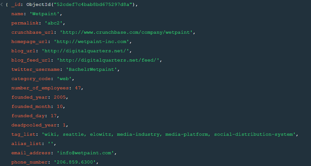
We’ll consider an example to understand how Bayesian Thinking is used to make sound decisions.

For the sake of simplicity, let’s imagine a management consultation firm hires only two types of employees. Let’s say, IT professionals and business consultants. You come across an employee of this firm, let’s call him Raj. You notice something about Raj instantly. Raj is shy. Now if you were asked to guess which type of employee Raj is what would be your guess?

If your guess is that Raj is an IT guy based on shyness as an attribute, then you have already fallen for one of the inherent cognitive biases. We’ll talk more about it later. But what if it can be proved Raj is actually twice as likely to be a Business Consultant?!

This is where Bayesian Thinking allows us to keep account of priors and likelihood information to predict a posterior probability.

The inherent cognitive bias you fell for is actually called – Base Rate Neglect. Base Rate Neglect occurs when we do not take into account the underlying proportion of a group in the population. Put it simply, what is the proportion of IT professionals to Business consultants in a business management firm? It would be fair to assume for every 1 IT professional, the firm hires 10 business consultants.

Another assumption could be made about shyness as an attribute. It would be fair to assume shyness is more common in IT professionals as compared to business consultants. Let’s assume, 75% of IT professionals are in fact shy corresponding to about 15% of business consultants.

Think of the proportion of employees in the firm as the prior odds. Now, think of the shyness as an attribute as the Likelihood. The figure below demonstrates when we take a product of the two, we get posterior odds.

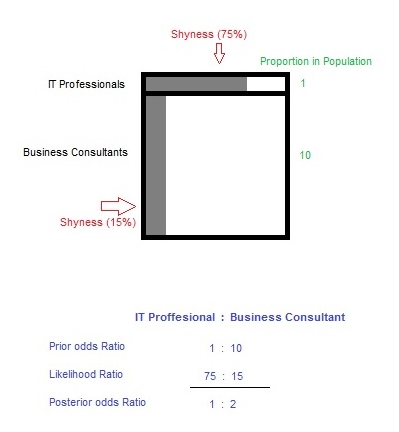
Plugging in the values shows us that Raj is actually twice as likely to be a Business consultant. This proves to us that by applying Bayesian Thinking we can eliminate bias and make a sound judgment.

Now, it would be unrealistic for you to try drawing a diagram or quantifying assumptions in most of the cases. So, how do we learn to apply Bayesian Thinking without quantifying our assumptions? Turns out we could, if we understood what are the underlying principles of Bayesian Thinking are.

Principles of Bayesian Thinking

Rule 1 – Remember your priors!

As we saw earlier how easy it is to fall for the base rate neglect trap. The underlying proportion in the population is often times neglected and we as human beings have a tendency to just focus on just the attribute. Think of priors as the underlying or the background knowledge which is essentially an additional bit of information in addition to the likelihood. A product of the priors together with likelihood determines the posterior odds/probability.

Rule 2 – Question your existing belief

This is somewhat tricky and counter-intuitive to grasp but question your priors. Present yourself with a hypothesis what if your priors were irrelevant or even wrong? How will that affect your posterior probability? Would the new posterior probability be any different than the existing one if your priors are irrelevant or even wrong?

Rule 3 – Update incrementally

We live in a dynamic world where evidence and attributes are constantly shifting. While it is okay to believe in well-tested priors and likelihoods in the present moment. However, always question does my priors & likelihood still hold true today? In other words, update your beliefs incrementally as new information or evidence surfaces. A good example of this would be the shifting sentiments of the financial markets. What holds true today, may not tomorrow? Hence, the priors and likelihoods must also be incrementally updated.

Conclusion

In conclusion, Bayesian Thinking is a powerful tool to hone your judgment skills. Developing Bayesian Thinking essentially tells us what to believe in and how much confident you are about that belief. It also allows us to shift our existing beliefs in light of new information or as the evidence unfolds. Hopefully, you now have a better understanding of Bayesian Thinking and why is it so important.

On that note, we would like to say DexLab Analytics is a premium data analytics training institute located in the heart of Delhi NCR. We provide intensive training on a plethora of data-centric subjects, including data science, Python and credit risk analytics. Stay tuned for more such interesting blogs and updates!

About the Author: Nish Lau Bakshi is a professional data scientist with an actuarial background and a passion to use the power of statistics to tackle various pressing, daily life problems.

Interested in a career in Data Analyst?
To learn more about Data Analyst with Advanced excel course – Enrol Now.
To learn more about Data Analyst with R Course – Enrol Now.
To learn more about Big Data Course – Enrol Now.
To learn more about Machine Learning Using Python and Spark – Enrol Now.
To learn more about Data Analyst with SAS Course – Enrol Now.
To learn more about Data Analyst with Apache Spark Course – Enrol Now.
To learn more about Data Analyst with Market Risk Analytics and Modelling Course – Enrol Now.

ANZ uses R programming for Credit Risk Analysis

Posted on March 10, 2017January 29, 2019 by Dexlab

At the previous month’s “R user group meeting in Melbourne”, they had a theme going; which was “Experiences with using SAS and R in insurance and banking”. In that convention, Hong Ooi from ANZ (Australia and New Zealand Banking Group) spoke on the “experiences in credit risk analysis with R”. He gave a presentation, which has a great story told through slides about implementing R programming for fiscal analyses at a few major banks.

In the slides he made, one can see the following:

How R is used to fit models for mortgage loss at ANZ

A customized model is made to assess the probability of default for individual’s loans with a heavy tailed T distribution for volatility.

One slide goes on to display how the standard lm function for regression is adapted for a non-Gaussian error distribution — one of the many benefits of having the source code available in R.

A comparison in between R and SAS for fitting such non-standard models

Mr. Ooi also notes that SAS does contain various options for modelling variance like for instance, SAS PROC MIXED, PRIC NLIN. However, none of these are as flexible or powerful as R. The main difference as per Ooi, is that R modelling functions return as object as opposed to returning with a mere textual output. This however, can be later modified and manipulated with to adapt to a new modelling situation and generate summaries, predictions and more. An R programmer can do this manipulation.

`Read Also: From dreams to reality: a vision to train the youngsters about big data analytics by the young entrepreneurs:`

We can use cohort models to aggregate the point estimates for default into an overall risk portfolio as follows:

A comparison in between R and SAS for fitting such non-standard models — Photo Coutesy of revolution-computing.typepad.com

He revealed how ANZ implemented a stress-testing simulation, which made available to business users via an Excel interface:

The primary analysis is done in r programming within 2 minutes usually, in comparison to SAS versions that actually took 4 hours to run, and frequently kept crashing due to lack of disk space. As the data is stored within SAS; SAS code is often used to create the source data…

While an R script can be used to automate the process of writing, the SAS code can do so with much simplicity around the flexible limitations of SAS.

`Read Also: Dexlab Analytics' Workshop on Sentiment Analysis of Twitter Data Using R Programming`

Comparison between use of R and SAS’s IML language to implement algorithms:

Mr. Ooi’s R programming code has a neat trick of creating a matrix of R list objects, which is fairly difficult to do with IML’s matrix only data structures.

He also discussed some of the challenges one ma face when trying to deploy open-source R in the commercial organizations, like “who should I yell at if things do now work right”.

And lastly he also discussed a collection of typically useful R resources as well.

For people who work in a bank and need help adopting R in the workflow, may make use of this presentation to get some knowledge about the same. And also feel free to get in touch with our in-house experts in R programming at DexLab Analytics, the premiere R programming training institute in India.

Ref – https://www.r-bloggers.com/how-anz-uses-r-for-credit-risk-analysis/

Interested in a career in Data Analyst?
To learn more about Data Analyst with Advanced excel course – Enrol Now.
To learn more about Data Analyst with R Course – Enrol Now.
To learn more about Big Data Course – Enrol Now.
To learn more about Machine Learning Using Python and Spark – Enrol Now.
To learn more about Data Analyst with SAS Course – Enrol Now.
To learn more about Data Analyst with Apache Spark Course – Enrol Now.
To learn more about Data Analyst with Market Risk Analytics and Modelling Course – Enrol Now.

Call us to know more

Gurgaon

+91 852 787 2444 / +91 85271 91444

Kolkata

+91 931 572 5902