In our previous blog we discussed about few of the basic functions of MQL like .find() , .count() , .pretty() etc. and in this blog we will continue to do the same. At the end of the blog there is a quiz for you to solve, feel free to test your knowledge and wisdom you have gained so far.
Given below is the list of functions that can be used for data wrangling:-
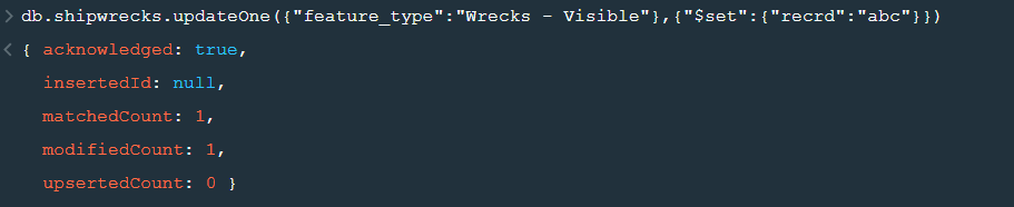
updateOne() :- This function is used to change the current value of a field in a single document.
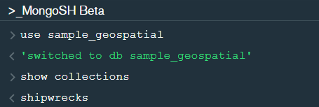
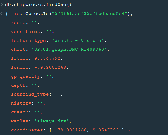
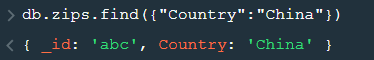
After changing the database to “sample_geospatial” we want to see what the document looks like? So for that we will use .findOne() function.
Now lets update the field value of “recrd” from ‘ ’ to “abc” where the “feature_type” is ‘Wrecks-Visible’.
Now within the .updateOne() funtion any thing in the first part of { } is the condition on the basis of which we want to update the given document and the second part is the changes which we want to make. Here we are saying that set the value as “abc” in the “recrd” field . In case you wanted to increase the value by a certain number ( assuming that the value is integer or float) you can use “$inc” instead.
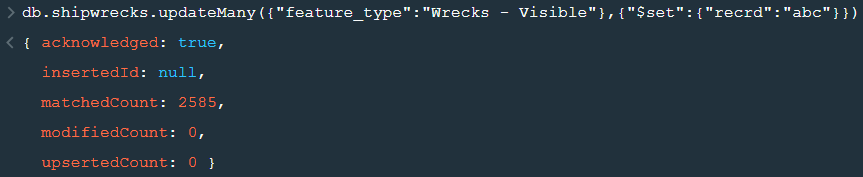
2. updateMany() :- This function updates many documents at once based on the condition provided.
3. deleteOne() & deleteMany() :- These functions are used to delete one or many documents based on the given condition or field.
4. Logical Operators :-
“$and” : It is used to match all the conditions.
“$or” : It is used to match any of the conditions.
The first code matches both the conditions i.e. name should be “Wetpaint” and “category_code” should be “web”, whereas the second code matches any one of the conditions i.e. either name should be “Wetpaint” or “Facebook”. Try these codes and see the difference by yourself.
So, with that we come to the end of the discussion on the MongoDB Basics. Hopefully it helped you understand the topic, for more information you can also watch the video tutorial attached down this blog. The blog is designed and prepared by Niharika Rai, Analytics Consultant, DexLab AnalyticsDexLab Analytics offers machine learning courses in Gurgaon. To keep on learning more, follow DexLab Analytics blog.
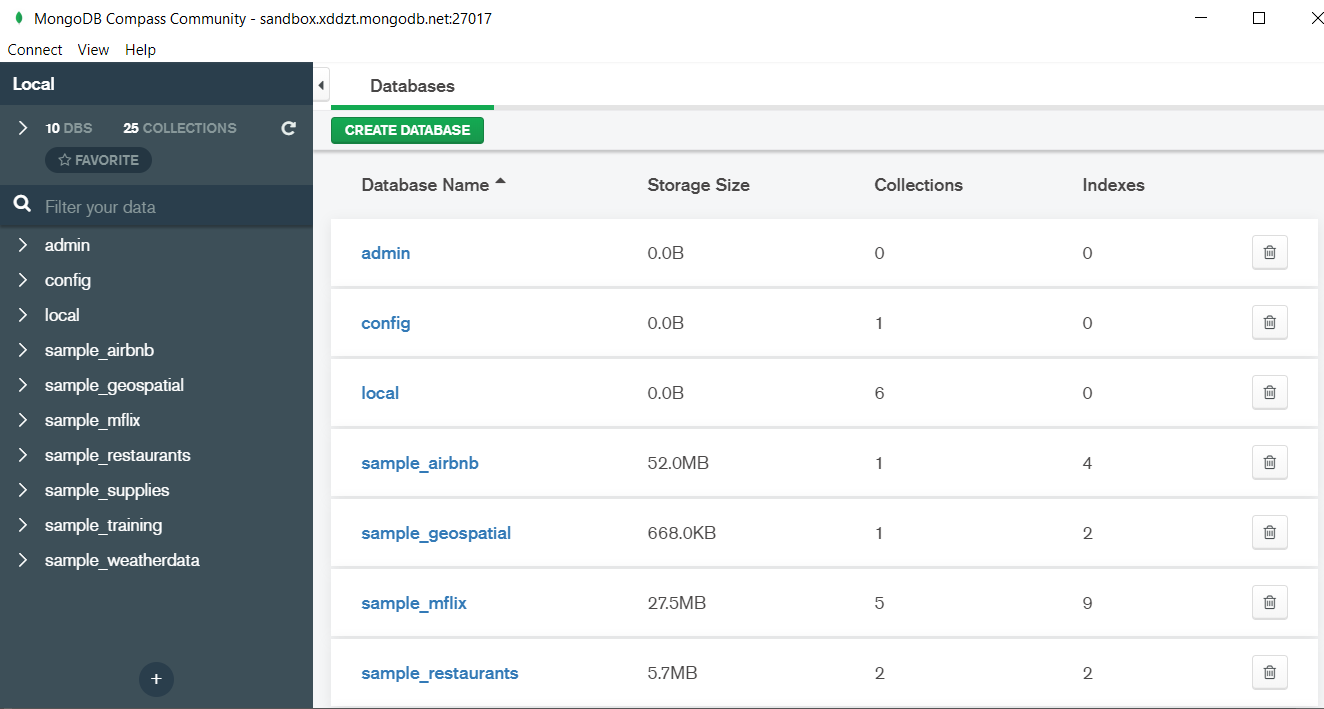
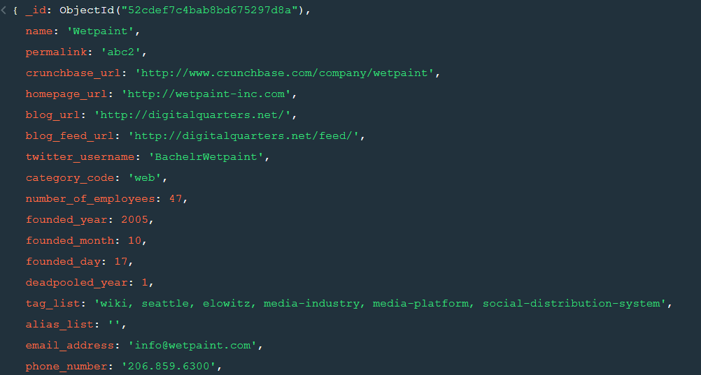
MongoDB is a document based database program which was developed by MongoDB Inc. and is licensed under server side public license (SSPL). It can be used across platforms and is a non-relational database also known as NoSQL, where NoSQL means that the data is not stored in the conventional tabular format and is used for unstructured data as compared to SQL and that is the major difference between NoSQL and SQL. MongoDB stores document in JSON or BSON format. JSON also known as JavaScript Object notation is a format where data is stored in a key value pair or array format which is readable for a normal human being whereas BSON is nothing but the JSON file encoded in the binary format which is quite hard for a human being to understand. Structure of MongoDB which uses a query language MQL(Mongodb query language):- Databases:- Databases is a group of collections. Collections:- Collection is a group fields. Fields:- Fields are nothing but key value pairs Just for an example look at the image given below:-
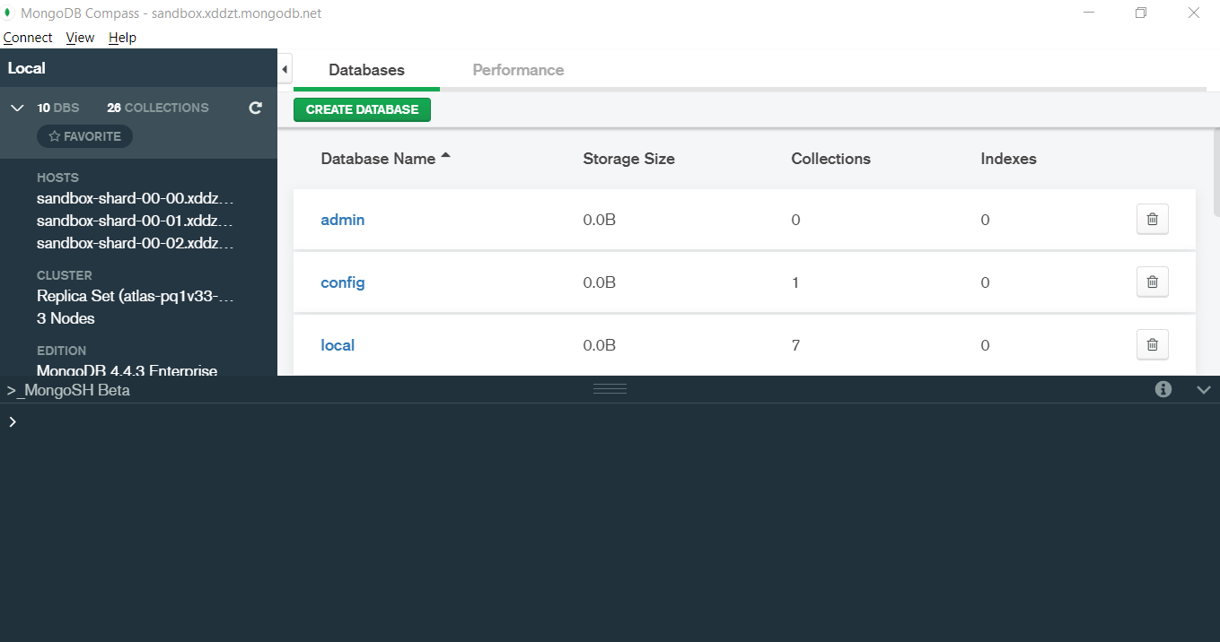
Here I am using MongoDB Compass a tool to connect to Atlas which is a cloud based platform which can help us write our queries and start performing all sort of data extraction and deployment techniques. You can download MongoDB Compass via the given link https://www.mongodb.com/try/download/compass
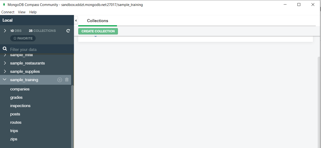
In the above image in the red box we have our databases and if we click on the “sample_training” database we will see a list of collections similar to the tables in sql.
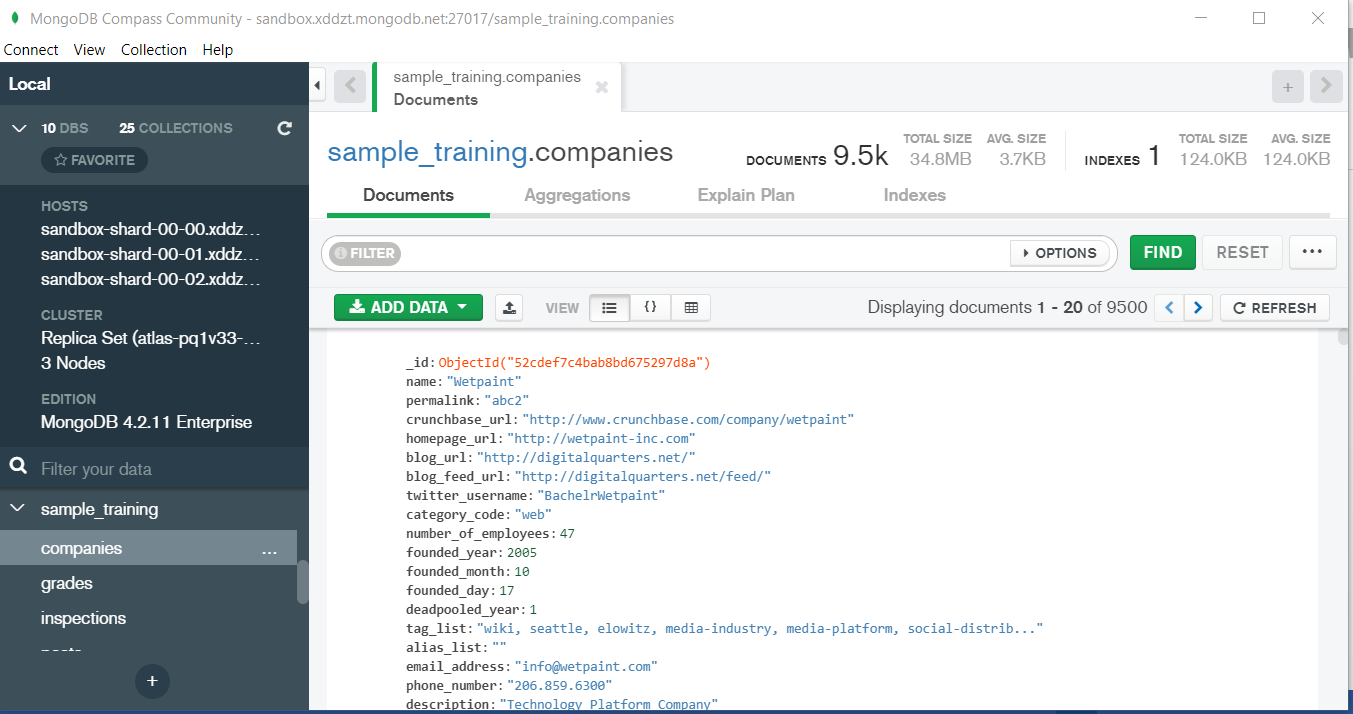
Now lets write our first query and see what data in “companies” collection looks like but before that select the “companies” collection.
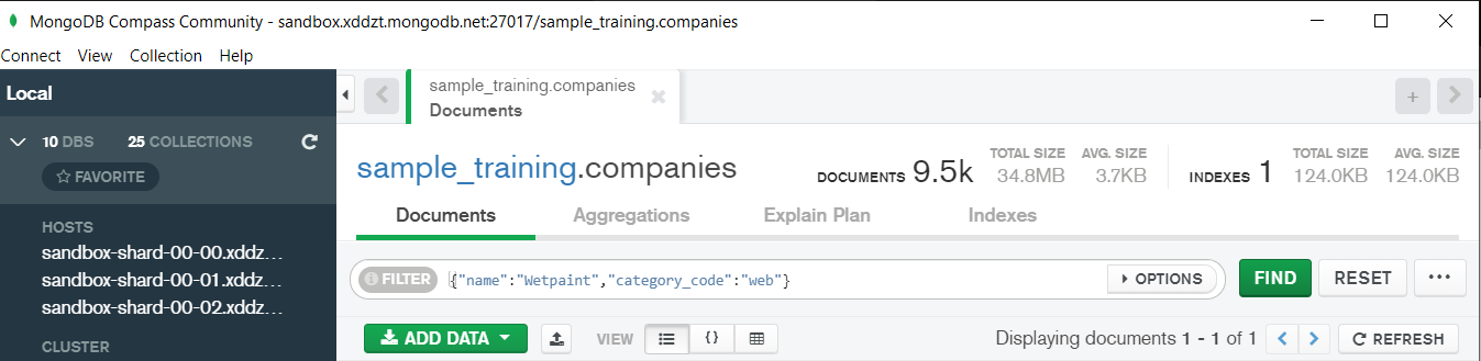
Now in our filter cell we can write the following query:-
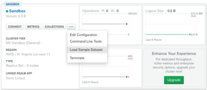
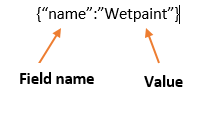
In the above query “name” and “category_code” are the key values also known as fields and “Wetpaint” and “web” are the pair values on the basis of which we want to filter the data. What is cluster and how to create it on Atlas? MongoDB cluster also know as sharded cluster is created where each collection is divided into shards (small portions of the original data) which is a replica set of the original collection. In case you want to use Atlas there is an unpaid version available with approximately 512 mb space which is free to use. There is a pre-existing cluster in MongoDB named Sandbox , which currently I am using and you can use it too by following the given steps:- 1. Create a free account or sign in using your Google account on https://www.mongodb.com/cloud/atlas/lp/try2-in?utm_source=google&utm_campaign=gs_apac_india_search_brand_atlas_desktop&utm_term=mongodb%20atlas&utm_medium=cpc_paid_search&utm_ad=e&utm_ad_campaign_id=6501677905&gclid=CjwKCAiAr6-ABhAfEiwADO4sfaMDS6YRyBKaciG97RoCgBimOEq9jU2E5N4Jc4ErkuJXYcVpPd47-xoCkL8QAvD_BwE 2. Click on “Create an Organization”. 3. Write the organization name “MDBU”. 4. Click on “Create Organization”. 5. Click on “New Project”. 6. Name your project M001 and click “Next”. 7. Click on “Build a Cluster”. 8. Click on “Create a Cluster” an option under which free is written. 9. Click on the region closest to you and at the bottom change the name of the cluster to “Sandbox”. 10. Now click on connect and click on “Allow access from anywhere”. 11. Create a Database User and then click on “Create Database User”. username: m001-student password: m001-mongodb-basics 12. Click on “Close” and now load your sample as given below :
Loading may take a while…. 13. Click on collections once the sample is loaded and now you can start using the filter option in a similar way as in MongoDB Compass In my next blog I’ll be sharing with you how to connect Atlas with MongoDB Compass and we will also learn few ways in which we can write query using MQL.
So, with that we come to the end of the discussion on the MongoDB. Hopefully it helped you understand the topic, for more information you can also watch the video tutorial attached down this blog. The blog is designed and prepared by Niharika Rai, Analytics Consultant, DexLab AnalyticsDexLab Analytics offers machine learning courses in Gurgaon. To keep on learning more, follow DexLab Analytics blog.
In this particular blog we will discuss about few of the basic functions of MQL (MongoDB Query Language) and we will also see how to use them? We will be using MongoDB Compass shell (MongoSH Beta) which is available in the latest version of MongoDB Compass.
Connect your Atlas cluster to your MongoDB Compass to get started. Latest version of MongoDB Compass will have this shell, so if you don’t find this shell then please install the latest version for this to work.
Now lets start with the functions.
find() :- You need this function for data extraction in the shell.
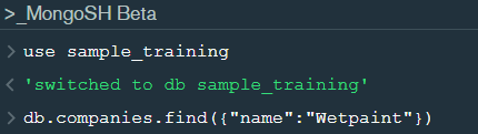
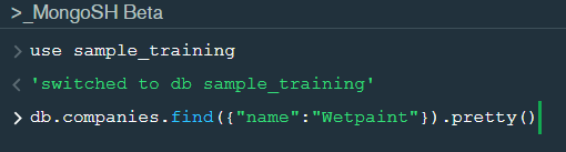
In the shell we need to first write the “use database name” code to access the database then use .find() to extract data which has name “Wetpaint”
For the above query we get the following result:-
The above result brings us to another function .pretty() .
2. pretty() :- this function helps us see the result more clearly.
Try it yourself to compare the results.
3. count() :- Now lets see how many entries we have by the company name “Wetpaint”.
So we have only one document.
4. Comparison operators :-
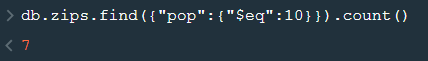
“$eq” : Equal to
“$neq”: Not equal to
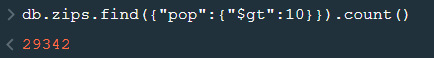
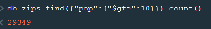
“$gt”: Greater than
“$gte”: Greater than equal to
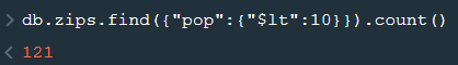
“$lt”: Less than
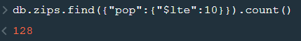
“$lte”: Less than equal to
Lets see how this works.
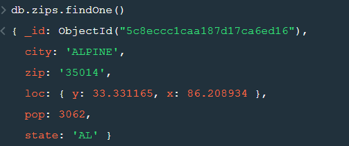
5. findOne() :- To get a single document from a collection we use this function.
6. insert() :- This is used to insert documents in a collection.
Now lets check if we have been able to insert this document or not.
Notice that a unique id has been added to the document by default. The given id has to be unique or else there will be an error. To provide a user defined id use “_id”.
So, with that we come to the end of the discussion on the MongoDB. Hopefully it helped you understand the topic, for more information you can also watch the video tutorial attached down this blog. The blog is designed and prepared by Niharika Rai, Analytics Consultant, DexLab AnalyticsDexLab Analytics offers machine learning courses in Gurgaon. To keep on learning more, follow DexLab Analytics blog.
This is another blog added to the series of time series forecasting. In this particular blog I will be discussing about the basic concepts of ARIMA model.
So what is ARIMA?
ARIMA also known as Autoregressive Integrated Moving Average is a time series forecasting model that helps us predict the future values on the basis of the past values. This model predicts the future values on the basis of the data’s own lags and its lagged errors.
When a data does not reflect any seasonal changes and plus it does not have a pattern of random white noise or residual then an ARIMA model can be used for forecasting.
There are three parameters attributed to an ARIMA model p, q and d :-
p :- corresponds to the autoregressive part
q:- corresponds to the moving average part.
d:- corresponds to number of differencing required to make the data stationary.
In our previous blog we have already discussed in detail what is p and q but what we haven’t discussed is what is d and what is the meaning of differencing (a term missing in ARMA model).
Since AR is a linear regression model and works best when the independent variables are not correlated, differencing can be used to make the model stationary which is subtracting the previous value from the current value so that the prediction of any further values can be stabilized . In case the model is already stationary the value of d=0. Therefore “differencing is the minimum number of deductions required to make the model stationary”. The order of d depends on exactly when your model becomes stationary i.e. in case the autocorrelation is positive over 10 lags then we can do further differencing otherwise in case autocorrelation is very negative at the first lag then we have an over-differenced series.
The formula for the ARIMA model would be:-
To check if ARIMA model is suited for our dataset i.e. to check the stationary of the data we will apply Dickey Fuller test and depending on the results we will using differencing.
In my next blog I will be discussing about how to perform time series forecasting using ARIMA model manually and what is Dickey Fuller test and how to apply that, so just keep on following us for more.
So, with that we come to the end of the discussion on the ARIMA Model. Hopefully it helped you understand the topic, for more information you can also watch the video tutorial attached down this blog. The blog is designed and prepared by Niharika Rai, Analytics Consultant, DexLab AnalyticsDexLab Analytics offers machine learning courses in Gurgaon. To keep on learning more, follow DexLab Analytics blog.
ARMA(p,q) model in time series forecasting is a combination of Autoregressive Process also known as AR Process and Moving Average (MA) Process where p corresponds to the autoregressive part and q corresponds to the moving average part.
Autoregressive Process (AR) :- When the value of Yt in a time series data is regressed over its own past value then it is called an autoregressive process where p is the order of lag into consideration.
Where,
Yt = observation which we need to find out.
α1= parameter of an autoregressive model
Yt-1= observation in the previous period
ut= error term
The equation above follows the first order of autoregressive process or AR(1) and the value of p is 1. Hence the value of Yt in the period ‘t’ depends upon its previous year value and a random term.
Moving Average (MA) Process :- When the value of Yt of order q in a time series data depends on the weighted sum of current and the q recent errors i.e. a linear combination of error terms then it is called a moving average process which can be written as :-
yt = observation which we need to find out
α= constant term
βut-q= error over the period q .
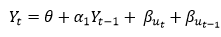
ARMA (Autoregressive Moving Average) Process :-
The above equation shows that value of Y in time period ‘t’ can be derived by taking into consideration the order of lag p which in the above case is 1 i.e. previous year’s observation and the weighted average of the error term over a period of time q which in case of the above equation is 1.
How to decide the value of p and q?
Two of the most important methods to obtain the best possible values of p and q are ACF and PACF plots.
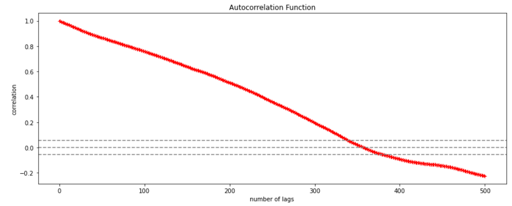
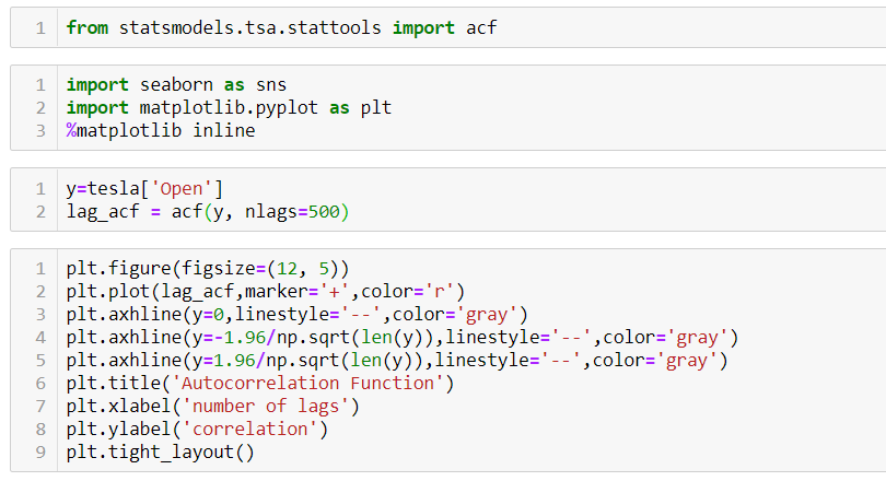
ACF (Auto-correlation function) :- This function calculates the auto-correlation of the complete data on the basis of lagged values which when plotted helps us choose the value of q that is to be considered to find the value of Yt. In simple words how many years residual can help us predict the value of Yt can obtained with the help of ACF, if the value of correlation is above a certain point then that amount of lagged values can be used to predict Yt.
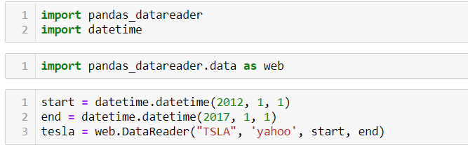
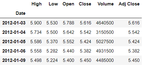
Using the stock price of tesla between the years 2012 and 2017 we can use the .acf() method in python to obtain the value of p.
.DataReader() method is used to extract the data from web.
The above graph shows that beyond the lag 350 the correlation moved towards 0 and then negative.
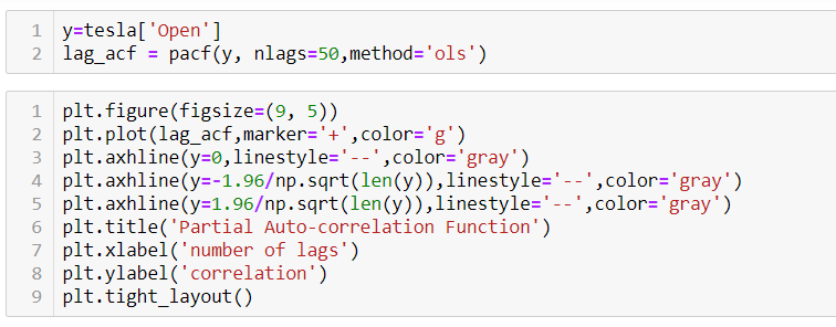
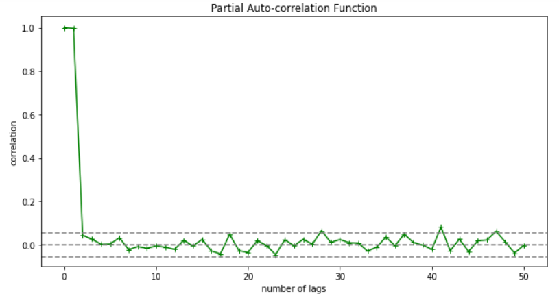
PACF (Partial auto-correlation function) :- Pacf helps find the direct effect of the past lag by removing the residual effect of the lags in between. Pacf helps in obtaining the value of AR where as acf helps in obtaining the value of MA i.e. q. Both the methods together can be use find the optimum value of p and q in a time series data set.
Lets check out how to apply pacf in python.
As you can see in the above graph after the second lag the line moved within the confidence band therefore the value of p will be 2.
So, with that we come to the end of the discussion on the ARMA Model. Hopefully it helped you understand the topic, for more information you can also watch the video tutorial attached down this blog. The blog is designed and prepared by Niharika Rai, Analytics Consultant, DexLab AnalyticsDexLab Analytics offers machine learning courses in Gurgaon. To keep on learning more, follow DexLab Analytics blog.
In this blog we will be introducing you to the Gaussian Distribution/Normal Distribution. Knowledge of the distribution of your data is quite important as it tells you the trend your data follows and a continuous observation of the trend helps you predict the future observations more accurately.
One of the most important distribution in statistics is Gaussian Distribution also known as Normal Distribution follows, that the mean, median and mode of the data are equal or almost equal. The idea behind this is that the data you collect should not have a very high standard deviation.
How to generate a normally distributed data in Python
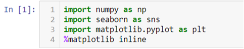
First we will import all the necessary libraries
Now we will use .normal() method from Numpy library to generate the data where 50 is the mean, .1 is the deviation and 500 is the number of observations to be generated.
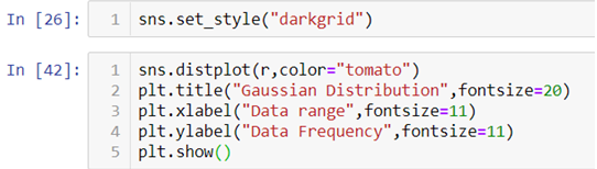
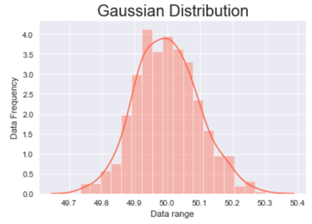
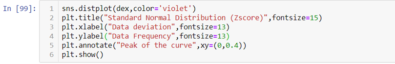
To plot the data and have a look at the data distribution we will be using .distplot() method from the Seaborn library and to make our plot visually better we will be using .set_style() method to change the background of our graph.
In the above line of codes we are also using Matplotlib library to add axis labels and title to the graph. We are also adding an argument fontsize to adjust the size of the font.
The above graph is a bell shaped curve with the peak of the curve in the center of the graph. This is one of the most important assumption of the Gaussian distribution on that the curve is symmetric at the center, some of the other assumptions are:-
Assumptions of the Gaussian distribution:
The mean, median and mode are equal.
Exactly half of the values are to the left of the center and exactly half of the values are to the right.
The total area under the curve is 1.
It has a continuous probability distribution.
68% of the data is -1 to 1 standard deviation away from the mean.
95% of the data is -2 to 2 standard deviation away from the mean.
99.7% of the data is -3 to 3 standard deviation away from the mean.
The last three assumptions can be proven with the help of standard normal distribution.
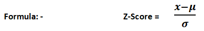
What is standard normal distribution?
Standard normal distribution also known as Z-score is a special case of normal distribution where we convert the normally distributed data into data deviations. The mean of such a distribution is 0 and the standard deviation is 1.
Let’s see how we can achieve the standard normal distribution in Python.
We will be using the same normally distributed data as above.
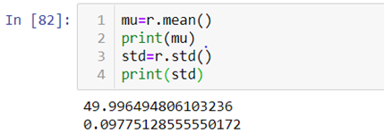
First we will be calculating the mean and standard deviation of the data we created with the help of the above code by using .mean() and .std() method.
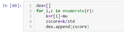
Now to calculate the Z-score we will first make an empty list and then append the calculated values one by one in that list with the help of a for-loop.
As you can see in the above code we are first subtracting the value from the mean and then dividing it by the standard deviation.
Now let’s see how the calculated data visually looks like.
When we look at the above graph we can clearly see that the data is by max 3 standard deviations away from the mean.
For further explanation check out the video attached down the blog.
So, with this we come to the end of today’s discussion on Gaussian distribution, hopefully, you found this explanation helpful. For such informative posts keep an eye on the Dexlab Analytics blog. Dexlab Analytics is a premier institute that offers cutting edge courses such as credit risk analysis course in Delhi.
When a lender starts a financial institution with the aim of lending money to entities, he is most strongly fortified against credit risk. He undertakes several measures to lower credit risk and this is called credit risk modelling.
“A good credit risk assessment can prevent avoidable losses for an organization. When a borrower is found to be a debtor, it could dent their creditworthiness. The lender will be skeptical about offering loans for fear of not getting it back,” says a report.
Credit risk assessment is done to gauge whether a borrower can pay back a loan. The credit risk of a consumer is determined by the five Cs – capacity to repay, associated collateral, credit history, capital, and the loan’s conditions.
“If a borrower’s credit risk is high, their loan’s interest rate will be increased. Credit risk shows the likelihood of a lender losing their loaned money to a borrower.”Credit risk highlights a borrower’s ability to honour his contractual agreements and repay loans.
“Conventionally, it deals with the risk every lender must be familiar with, which is losing the principal and interest owed. The aftermath of this is a disturbance to the lender’s cash flow and the possibility of losing more money in a bid to recover the loan.”
Credit Risk Modelling
While there is no pronounced way to determine the credit risk of an individual, credit risk modeling is an instrument that has largely come to be used by financial institutions to accurate measure credit risk.
“Credit risk modeling involves the use of data models to decide on two important issues. The first calculates the possibility of a default on the part of a loan borrower. The second determines how injurious such default will be on the lender’s financial statement.”
Financial Statement Analysis Models
Popular examples of these models include Moody’s RiskCalc and Altman Z-score. “The financial statements obtained from borrowing institutions are analyzed and then used as the basis of these models.”
Default Probability Models
The Merton model is a suitable example of this kind of credit risk modeling. The Merton model is also a structural model. Models like this take into account a company’s capital structure “because it is believed here that if the value of a company falls below a certain threshold, then the company is bound to fail and default on its loans”.
Machine Learning Models
“The influence of machine learning and big data on credit risk modeling has given rise to more scientific and accurate credit risk models. One example of this is the Maximum Expected Utility model.”
The 5Cs of Credit Risk Evaluation
These are quantitative and qualitative methods adopted for the evaluation of a borrower.
Character
“This generally looks into the track record of a borrower to know their reputation in the aspect of loan repayment.”
Capacity
“This takes the income of the borrower into consideration and measures it against their recurring debt. This also delves into the borrower’s debt-to-income (DTI) ratio.”
Capital
The amount of money a borrower is willing to contribute to a potential project can determine if the lender will lend him money.
Collateral
“It gives the lender a win-win situation, in the sense that upon a default, the lender can sell the collateral to recover the loan.”
Conditions
“This takes information such as the amount of principal and interest rate into consideration for a loan application. Another factor that can be considered as conditions is the reason for the loan.”
Conclusion
There is no formula anywhere that exposes the borrower who is going to default on loan repayment. However, the proper assessment of credit risk can go a long way in reducing the impact of a loss on a lender. For more on this, do visit the DexLab Analytics website today. DexLab Analtyics is a premiere institute that provides credit risk analysis courses online.
Credit Risk Modeling is the analysis of the credit risk of a borrower. It helps in understanding the risk, which a lender may face when he offers a credit.
What is Credit Risk?
Credit risk is the risk involved in any kind of loan. In other words, it is the risk that a lender runs when he lends a sum to somebody. It is thus, the risk of not getting back the principal sum or the interests of it on time. Suppose, a person is lending a sum to his friend, then the credit risk models will help him to assess the probability of timely payments and estimate the total loss in case of defaulters.
Credit Risk Modelling and its Importance
In the fast-paced world of now, a loss cannot be afforded at any cost. Here’s where the Credit Risk Modeling steps in. It primarily benefits the lenders by accurate approximation of the credit risk of a borrower and thereby, cutting the losses short.
Credit Risk Modelling is extensively used by financial institutions around the world to estimate the credit risk of potential borrowers. It helps them in calculating the interest rates of the loans and also deciding on whether they would grant a particular loan or not.
The Changing Models for the Analysis of Credit Risks
With the rapid progress of technology, the traditional models of credit risks are giving way to newer models using R and Python. Moreover, credit risk modeling using the state-of-the-art tools of analytics and Big Data are gaining huge popularity.
Along with the changing technology, the advancing economies and the successive emergence of a range of credit risks have also transformed the credit risk models of the past.
What Affects Credit Risk Modeling?
A lender runs a varying range of risks from disruption of cash flows to a hike in the collection costs, from the loss of interest/interests to losing the whole sum altogether. Thus, Credit Risk Modelling is paramount in importance at this age we are living. Therefore, the process of assessing credit risk should be as exact as feasible.
However, in this process, there are 3 main factors that regulate the risk of the credit of the borrowers. Here they are:
The Probability of Default (PD) – This refers to the possibility of a borrower defaulting a loan and is thus, a significant factor to be considered when modeling credit risks. For the individuals, the PD score is modeled on the debt-income ratio and existing credit score. This score helps in figuring out the interest rates and the amount of down payment.
Loss Given Default (LGD) – The Loss Given Default or LGD is the estimation of the total loss that the lender would incur in case the debt remains unpaid. This is also a critical parameter that you should weigh before lending a sum. For instance, if two different borrowers are borrowing two different sums, the credit risk profiles of the borrower with a large sum would vary greatly to the other, who is borrowing a much smaller sum of money, even though their credit score and debt-income ratio match exactly with each other.
Exposure at Default (EAD) – EAD helps in calculating the total exposure that a lender is subjected to at any given point in time. This is also a significant factor exposing the risk appetite of the lender, which considerably affects the credit risk.
Endnotes
Though credit risk assessment seems like a tough job to assume the repayment of a particular loan and its defaulters, it is a peerless method which will give you an idea of the losses that you might incur in case of delayed payments or defaulters.
Risk is an intrinsic part of the money lending system. There’s always the chance that customers borrowing money from financial institutions fail to repay their loans. And to determine the exact probability of a customer paying off a loan or defaulting on it, banks and other lenders rely on credit risk modeling.
Next-Gen Credit Assessment Techniques
The credit situation has changed a lot from how it used to be ten years ago. And to keep up, lenders must also evolve by identifying and responding to issues in real-time. Credit risk strategy has become more complex and multiple factors need to be weighed to arrive at the correct decision that’s both profitable for the enterprise and customer. Sophisticated models that contain more than one dimension, such as additional information about a customer’s finance and behavior patterns, are in demand. These models help get a 360 degree view of the customer’s financial condition.
Moreover, banks want to provide broader financial inclusion with the intention that more customers get credit scores and avail their financial services. But they need to keep a check on their risk levels too. Traditional credit assessment techniques having linear nature, for example logistic regression, are useful, but only till a point.
Neural Networks
Recent developments in neural networks have greatly improved credit risk modeling and seem to provide a solution to the above mentioned problem. One such breakthrough is the NeuroDecision Technology from Equifax that facilitates more inclusive models, so scores and consent can be given to a bigger and varied group of customers.
Machine Learning (ML) is a fast-moving field and neural networks are used within deep learning, which is an advanced form of ML. It has the potential to make more accurate predictions and go beyond the linear analysis methods of logistic regression. This is a positive development for both the business and its customers.
Linear Vs. Inclusive
What happens in a logistic regression model is that all customers above a straight line (prime) get approved, whereas everyone falling below that line (subprime) gets rejected. Hence, customers who are working hard towards creating a good credit profile but fall just below prime get declined repeatedly. Despite this problem, traditional linear models are widely used because outcomes can be easily conveyed to customers, which helps to be in sync with consumer credit regulations that demand higher transparency.
On the other hand, neural networks lead to non-linear or curved arcs that include those customers who aren’t yet prime, but are evidently moving in the right direction. This increases the ‘approved customer’ base, which is beneficial for the business because customers are being served better and the enterprise is growing. This model is advantageous from the perspective of customers also as it allows more people to access mainstream financial services. The only problem is explaining the outcome to customers as neural networks tend to be rather complex.
Concluding Note
Many companies are producing robust credit modeling tools employing deep learning techniques. And these game-changing developments highlight the fact that they are just the starting point of a series of interesting developments ahead.