
In this post, we will discuss how to use the package nmle in R programming, which includes the dataset MathArchieve. To install the package and load it into your R programming environment, use the code mentioned below:
####################################################
#code for visual large dataset MathAchieve
#first show 3d scatterplot; then show tableplot variations
####################################################
install.packages(“nmle”) #install nmle package
library(nlme) #load the package into the R environment
####################################################
After you install the package, just take a quick look at the structure of the dataset by making use of the following code:
####################################################
attach(MathAchieve) #take a look at the structure of the dataset
str(MathAchieve)
####################################################
Classes ‘nfnGroupedData’, ‘nfGroupedData’, ‘groupedData’ and ‘data.frame’: 7185 obs. of 6 variables:
$ School : Ord.factor w/ 160 levels “8367”<“8854″<..: 59 59 59 59 59 59 59 59 59 59 …
$ Minority: Factor w/ 2 levels “No”,”Yes”: 1 1 1 1 1 1 1 1 1 1 …
$ Sex : Factor w/ 2 levels “Male”,”Female”: 2 2 1 1 1 1 2 1 2 1 …
$ SES : num -1.528 -0.588 -0.528 -0.668 -0.158 …
$ MathAch : num 5.88 19.71 20.35 8.78 17.9 …
$ MEANSES : num -0.428 -0.428 -0.428 -0.428 -0.428 -0.428 -0.428 -0.428 -0.428 -0.428 …
– attr(*, “formula”)=Class ‘formula’ language MathAch ~ SES | School
.. ..- attr(*, “.Environment”)=<environment: R_GlobalEnv>
– attr(*, “labels”)=List of 2
..$ y: chr “Mathematics Achievement score”
..$ x: chr “Socio-economic score”
– attr(*, “FUN”)=function (x)
..- attr(*, “source”)= chr “function (x) max(x, na.rm = TRUE)”
– attr(*, “order.groups”)= logi TRUE
>
As can be noted from the above mentioned above the MathAchieve data set includes somewhere around 7185 observations and six variables. Three of these variables are numeric and three others are the factors. Thus, this offers some obstacles when we try to visualize the data. With more than 7000 cases and a 2-D scatterplot, thus displaying bivariate correlations among the 3 numerical variable which is limited to utility.

We can make use of a 3-dimensional scatterplot and a linear regression model to visualize more clearly and dissect the relationships among the three numeric variables.
The variable SES is in fact a vector that measures the socio-economic status, MathAch is a numerical vector which calculates the mathematical achievement scores, and MEANSES is a vector which calculates the mean SES for the school attended by every student given in the sample.
Here s how we can look at the correlation matrix for these 3 variables, to get a good sense of th relationships among the variables:
> ####################################################
> #do a correlation matrix with the 3 numeric vars;
> ###################################################
> data(“MathAchieve”)
> cor(as.matrix(MathAchieve[c(4,5,6)]), method=”pearson”)
SES MathAch MEANSES
SES 1.0000000 0.3607556 0.5306221
MathAch 0.3607556 1.0000000 0.3437221
MEANSES 0.5306221 0.3437221 1.0000000
>
For using the cor() function, as is shown above we can understand the variables that have been used by specifying the column that each numeric variable is in as is shown in the output from the str() function.
The three numeric variables, for instance, are in the columns 4, 5, and 6 mentioned in the matrix.
As we have discussed previously in other tutorials, we can visualize the relationship among these three variables with the use of a three dimensional scatterplot. To do so, use the code mentioned below:
####################################################
#install.packages(“nlme”)
install.packages(“scatterplot3d”)
library(scatterplot3d)
library(nlme) #load nmle package
attach(MathAchieve) #MathAchive dataset is in environment
scatterplot3d(SES, MEANSES, MathAch, main=”Basic 3D Scatterplot”) #do the plot with default options
####################################################
We are the leading R programming training institute in Delhi NCR with a newly opened branch in Pune, feel free to contact us for any queries related to R programming and data analytics.
The resulting output plot will be as given below:
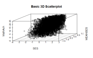
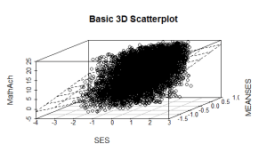
While having the scatterplot lacks detail due to the large sample size it is still possible to witness the medial correlations that are displayed in the correlation matrix by noting the shape and the direction of the data points. A regression plane can be evaluated and then added to the plot using the below mentioned code:
scatterplot3d(SES, MEANSES, MathAch, main=”Basic 3D Scatterplot”) #do the plot with default options
####################################################
##use a linear regression model to plot a regression plane
#y=MathAchieve, SES, MEANSES are predictor variables
####################################################
model1=lm(MathAch ~ SES + MEANSES) ## generate a regression
#take a look at the regression output
summary(model1)
#run scatterplot again putting results in model
model <- scatterplot3d(SES, MEANSES, MathAch, main=”Basic 3D Scatterplot”) #do the plot with default options
#link the scatterplot and linear model using the plane3d function
model$plane3d(model1) ## link the 3d scatterplot in ‘model’ to the ‘plane3d’ option with ‘model1’ regression information
####################################################
The output that will result can be seen as is mentioned below:
Call:
lm(formula = MathAch ~ SES + MEANSES)
Residuals:
Min 1Q Median 3Q Max
-20.4242 -4.6365 0.1403 4.8534 17.0496
Coefficients:
Estimate Std. Error t value Pr(>|t|)
(Intercept) 12.72590 0.07429 171.31 <2e-16 ***
SES 2.19115 0.11244 19.49 <2e-16 ***
MEANSES 3.52571 0.21190 16.64 <2e-16 ***
—
Signif. codes: 0 ‘***’ 0.001 ‘**’ 0.01 ‘*’ 0.05 ‘.’ 0.1 ‘ ’ 1
Residual standard error: 6.296 on 7182 degrees of freedom
Multiple R-squared: 0.1624, Adjusted R-squared: 0.1622
F-statistic: 696.4 on 2 and 7182 DF, p-value: < 2.2e-16
The plot with the plane obtained is seen as:
Though the above analysis gives us several useful insights, it remains limited by the mixture of numeric values and factors. A more detail-oriented visual analysis which will enable us the display and comparison of all six of the variables which is possible by using the functions available in the R package Tableplots. This package was built to help in the visualization and observation, of large datasets with several variables.
The MathAchieve includes six variables in total, and 7185 cases as well. And the Tableplots package can be used with datasets that are larger than 10,000 observations and are up to 12 or so variables.
They can utilized to visualize relationships among variables using the same calculation scale or a mixed measurement types.
In order to take a look at the comparisons of each data type and then view all of the 6 together you must start with the following code:
####################################################
attach(MathAchieve) #attach the dataset
#set up 3 data frames with numeric, factors, and mixed
####################################################
mathmix <- data.frame(SES,MathAch,MEANSES,School=factor(School),Minority=factor(Minority),Sex=factor(Sex)) #all 6 vars
mathfact <- data.frame(School=factor(School),Minority=factor(Minority),Sex=factor(Sex)) #3 factor vars
mathnum <- data.frame(SES,MathAch,MEANSES) #3 numeric vars
####################################################
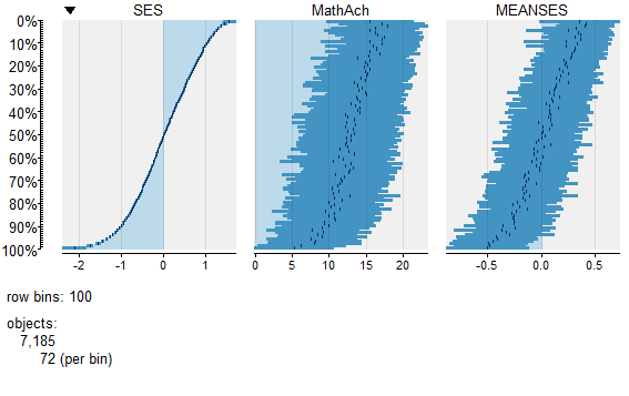
To view a comparison of the 3 numeric variables use:
####################################################
require(tabplot) #load tabplot package
tableplot(mathnum) #generate a table plot with numeric vars only
####################################################
And to view the comparison of the 3 numeric variable use the following:
####################################################
require(tabplot) #load tabplot package
tableplot(mathfact) #generate a table plot with factors only
####################################################
The final output will be as the following:
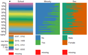
To view only the 3 factor variables use:
####################################################
require(tabplot) #load tabplot package
tableplot(mathfact) #generate a table plot with factors only
####################################################
This will result in the following:
To visualize and compare the table plots of all the six variables use the following:
####################################################
require(tabplot) #load tabplot package
tableplot(mathmix) #generate a table plot with all six variables
####################################################
Thereby, the resulting output to be as given below:
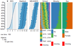
Making use of Tableplots can be very useful in visualizing relationships among a set of variables. the above given visual table comparisons agrees with the moderate correlation among the three numeric variables found in the correlation and the regression models which have discussed above.
To learn more about R programming certification in India, follow our regular updates on DexLab Analytics.
This post originally appeared on – www.r-bloggers.com/r-tutorial-visualizing-multivariate-relationships-in-large-datasets
Interested in a career in Data Analyst?
To learn more about Machine Learning Using Python and Spark – click here.
To learn more about Data Analyst with Advanced excel course – click here.
To learn more about Data Analyst with SAS Course – click here.
To learn more about Data Analyst with R Course – click here.
To learn more about Big Data Course – click here.
R Programming, R programming certification, R Programming Training, R Programming Tutorial