Python is an extremely readable and versatile high-level programming language. It supports both Object-oriented programming as well as Functional programming. It is generally referred to as an interpreted language which means that each line of code is executed one by one and if the interpreter finds an error it stops proceeding further and gives an error message to the user. This makes Python a widely regarded language, fueling Machine Learning Using Python, Text Mining with Python course and more. Furthermore, with such a high-end programming language, Python for data analysis looks ahead for a bright future.

In the Structure of Python
Computer languages have a structure just like human languages. Therefore, even in Python, we have comments, variables, literals, operators, delimiters, and keywords.
To understand the program structure of Python we will look at the following in this article: –
- Python Statement
- Simple Statement
- Compound Statement
- Multiple Statements Per Line
- Line Continuation
- Implicit Line Continuation
- Explicit Line Continuation
- Comments
- Whitespace
- Indentation
- Conclusion
Python Statement
A statement in Python is a logical instruction that the interpreter reads and executes. The interpreter executes statements sequentially, one by one. In Python, it could be an assignment statement or an expression. The statements are mostly written in such a style so that each statement occupies a single line.
Simple Statements
A simple statement is one that contains no other statements. Therefore, it lies entirely within a logical line. An assignment is a simple statement that assigns values to variables, unlike in some other languages; an assignment in Python is a statement and can never be part of an expression.
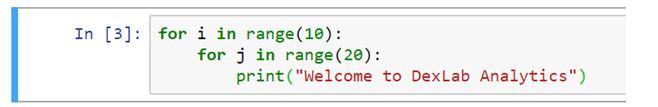
Compound Statement
A compound statement contains one or more other statements and controls their execution. A compound statement has one or more clauses, aligned at the same indentation. Each clause has a header starting with a keyword and ending with a colon (:), followed by a body, which is a sequence of one or more statements. When the body contains multiple statements, also known as blocks, these statements should be placed on separate logical lines after the header line, indented four spaces rightward.
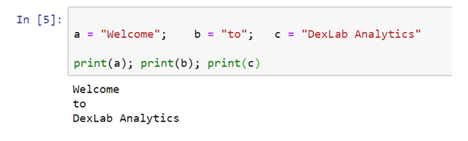
Multiple Statements per Line
Although it is not considered good practice multiple statements can be written in a single line in Python. It is advisable to avoid multiple statements in a single line. But, if it is necessary, then it can be written with the help of semicolon (;) as the terminator of every statement.
Line Continuation
In Python there might be some cases when a single statement is too long that does not fit the browser window and one needs to scroll the screen left or right. This can be a case of assignment statement with many terms or defining a lengthy nested list. These long statements of code are generally considered a poor practice.
To maintain readability, it is advisable to split the long statement into parts across several lines. In Python code, a statement can be continued from one line to the next in two different ways: implicit and explicit line continuation.
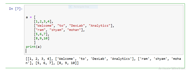
Implicit Line Continuation
This is the more straightforward technique for line continuation. In implicit line continuation, one can split a statement using either of parentheses ( ), brackets [ ] and braces { }. Here, one needs to enclose the target statement using the mentioned construct.
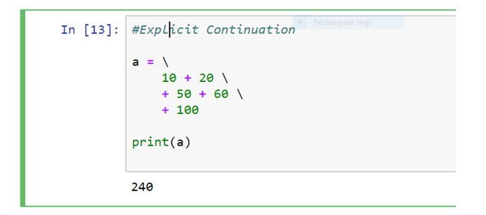
Explicit Line Continuation
In cases where implicit line continuation is not readily available or practicable, there is another option. This is referred to as an explicit line continuation or explicit line joining. Here, one can right away use the line continuation character (\) to split a statement into multiple lines.
Comments
A comment is text that doesn’t affect the outcome of a code; it is just a piece of text to let someone know what you have done in a program or what is being done in a block of code. This is especially helpful when a code is written and someone is analyzing it for bug fixing or making a change in logic, by reading a comment one can understand the purpose of code much faster than by just going through the actual code.
There are two types of comments in Python.
1. Single line comment
2. Multiple line comment
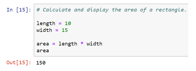
Single line comment
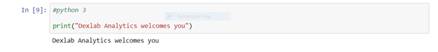
In python, one can use # special character to start the comment.
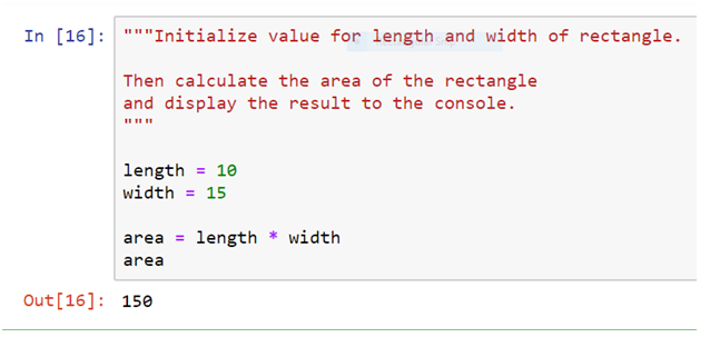
Multi-line comment
To have a multi-line comment in Python, one can use Triple Double Quotation at the beginning and the end of the comment.
Whitespace
One can improve the readability of the code with the use of whitespaces. Whitespaces are necessary for separating the keywords from the variables or other keywords. Whitespace is mostly ignored by the Python interpreter.
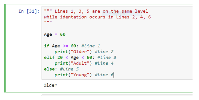
Indentation
Most of the programming languages provide indentation for better code formatting and don’t enforce to have it. However, in Python, it is mandatory to obey the indentation rules. Typically, we indent each line by four spaces (or by the same amount) in a block of code. Also for creating compound statements, the indentation will be of utmost necessity.
Conclusion
So, this article was all about how to structure the Python program. Here, one can learn what constitutes a valid Python statement and how to use implicit and explicit line continuation to write a statement that spans multiple lines. Furthermore, one can also learn about commenting Python code, and about the use of whitespace and indentation to enhance the overall readability.

We hope this article was helpful to y ou. If you are interested in similar blogs, stay glued to our website, and keep following all the news and updates from Dexlab Analytics.
Interested in a career in Data Analyst?
To learn more about Data Analyst with Advanced excel course – Enrol Now.
To learn more about Data Analyst with R Course – Enrol Now.
To learn more about Big Data Course – Enrol Now.To learn more about Machine Learning Using Python and Spark – Enrol Now.
To learn more about Data Analyst with SAS Course – Enrol Now.
To learn more about Data Analyst with Apache Spark Course – Enrol Now.
To learn more about Data Analyst with Market Risk Analytics and Modelling Course – Enrol Now.