Sas training institute Archives - Page 3 of 5 - DexLab Analytics | Big Data Hadoop SAS R Analytics Predictive Modeling & Excel VBA

INTCK and INTNX: All about SAS Dates and Computing Intervals between Dates

INTCK-and-INTNX

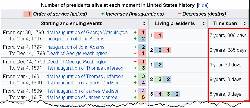
The INTCK and INTNX functions in SAS helps you compute the time between events. This technical blog is based on the timeline of living US presidents, sourced from a Wikipedia table. The table data shows the number of years and days between events.

So, let’s start.

LivingPresidents2

Gaps between dates

To calculate the interval between two dates, you can use these two SAS functions:

The INTCK function returns the number of time units between dates. The time unit can be selected in years, months, weeks, days, or whatever you feel like.

The INTNX function helps you compute the date that is 308 days away in the future from a specific date. This was just an example to help you understand what it means. The INTNX function returns a SAS date that is particular number of time units away from a particular date.

These two functions share a complimentary bond: where one calculates the difference between two dates, the other entitles you to add time units to a specified date value. Also, the INT part in both the functions denotes INTervals, and the terms INTCK and INTNX means Interval Check and Interval Next, respectively.

DexLab Analytics offers intensive SAS certification courses for candidates..

How to calculate anniversary dates

These two prime functions tend to be useful in counting the number of anniversaries between two dates along with calculating a future anniversary date. Use the ‘CONTINUOUS’ option for the INTCK function and the ‘SAME’ option for the INTNX function in the following manner:

The ‘CONTINUOUS’ option in the INTCK function helps you count the number of anniversaries of one date that occur before a second date. For example, the statement

Years = intck('year', '30APR1789'd, '04MAR1797'd, 'continuous');

returns the value 7 because there are 7 full years (anniversaries of 30APR) between those two dates. Without the ‘CONTINUOUS’ option, the function returns 8 as 01JAN occurs 8 times between those dates.

The statement

Anniv = intnx('year', '30APR1789'd, 7, 'same');

returns the 7th anniversary of the date 30APR1789. In some ways, it returns the date value for 30APR1796.

The most exciting part about these two functions is that they automatically handle leap years! Yes, you read that right. If you ask for the number of days within two dates, the INTCK function will show leap days in the result. If an event takes place on a leap day, and you ask the INTNX function to reveal the anniversary date, it will report 28FEB of the next year to the next anniversary date.

An algorithm calculating years and days between events

Go through the following algorithm to calculate the number of years and days between dates in SAS:

  • Use the INTCK function with the ‘CONTINUOUS’ option to calculate the number of completed years between two dates
  • Use the INTNX function to discover a third date, i.e. anniversary date, which is the same month and day like the start date, but takes place less than a year before the end date.
  • Use the INTCK function to ascertain the number of days occurring between the anniversary date and the end date.

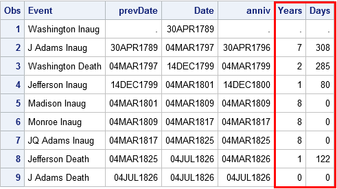
Here are the data steps that enable you to compute the time interval in years and days between the first few US presidential inaugurations and deaths.

data YearDays;
format Date prevDate anniv Date9.;
input @1  Date anydtdte12.
      @13 Event $26.;
prevDate = lag(Date);
if _N_=1 then do;                               /* when _N_=1, lag(Date)=. */
   Years=.; Days=.; return;            /* set years & days, go to next obs */
end;
Years = intck('year', prevDate, Date, 'continuous'); /* num complete years */
Anniv = intnx('year', prevDate, Years, 'same');      /* most recent anniv  */
Days = intck('day', anniv, Date);                    /* days since anniv   */
datalines;
Apr 30, 1789 Washington Inaug
Mar 4, 1797  J Adams Inaug
Dec 14, 1799 Washington Death
Mar 4, 1801  Jefferson Inaug
Mar 4, 1809  Madison Inaug
Mar 4, 1817  Monroe Inaug
Mar 4, 1825  JQ Adams Inaug
Jul 4, 1826  Jefferson Death
Jul 4, 1826  J Adams Death
run;
 
proc print data=YearDays;
var Event prevDate Date Anniv Years Days;
run;


LivingPresidents3


In a nutshell, the INTCK and INTNX functions are consequential for calculating intervals between dates. In this blog, I discussed about two-less-popular options inn SAS, for more such SAS training related blogs, follow us at DexLab Analytics.

Data Science Machine Learning Certification

This post originally appeared onblogs.sas.com/content/iml/2017/05/15/intck-intnx-intervals-sas.html
 

Interested in a career in Data Analyst?

To learn more about Machine Learning Using Python and Spark – click here.
To learn more about Data Analyst with Advanced excel course – click here.
To learn more about Data Analyst with SAS Course – click here.
To learn more about Data Analyst with R Course – click here.
To learn more about Big Data Course – click here.

The ABC of Summary Statistics and T Tests in SAS

The ABC of Summary Statistics and T Tests in SAS

Getting introduced to statistics for SAS training? Then, you must know how to create summary statistics (such as sample size, mean, and standard deviation) to test hypotheses and to figure confidence intervals. In this blog, we will show you how to furnish summary statistics (instead of raw data) to PROC TTEST in SAS, how to develop a data set that includes summary statistics and how to run PROC TTEST to calculate a two-sample or one-sample t test for the mean.

So, let’s start!

2

Running a two-sample t test for difference of means from summarized statistics

Instead of going the clichéd way, we will start with establishing a comparison between the mean heights of 19 students, based on gender – the data is held in the Sashelp class data set.

Observe the below SAS statements that sorts the data by the grouping variable, calling PROC MEANS and printing a subset of the statistics:

proc sort data=sashelp.class out=class; 
   by sex;                                /* sort by group variable */
run;
proc means data=class noprint;           /* compute summary statistics by group */
   by sex;                               /* group variable */
   var height;                           /* analysis variable */
   output out=SummaryStats;              /* write statistics to data set */
run;
proc print data=SummaryStats label noobs; 
   where _STAT_ in ("N", "MEAN", "STD");
   var Sex _STAT_ Height;
run;

summarystats1

The table reflects the structure of the Summary Stats set for two sample tests. The two samples used here are differentiated on the levels of the Sex Variable (‘F’ for females and ‘M’ for males). The _STAT_ column shows the name of the statistic implemented here. The Height column depicts the value of the statistics for individual group.

Get SAS certification Delhi from DexLab Analytics today!

The problem: The heights of sixth-grade students are normally distributed. Random samples of n1=9 females and n2=10 males are selected. The mean height of the female sample is m1=60.5889 with a standard deviation of s1=5.0183. The mean height of the male sample is m2=63.9100 with a standard deviation of s2=4.9379. Is there evidence that the mean height of sixth-grade students depends on gender?

Here, you have to do nothing special to get the PROC TTEST – whenever the procedure gets the sight of the respective variable _STAT_ and any unique values, the procedure understands that the data set comprises summarized statistics. The following representation compares the mean heights of males and females:

proc ttest data=SummaryStats order=data
           alpha=0.05 test=diff sides=2; /* two-sided test of diff between group means */
   class sex;
   var height;
run;

summarystats1

Check the confidence intervals for the standard deviations and also that the output includes 95% confidence intervals for group means.

In the second table, the ‘Pooled’ row radiates out the impression that both the variances of two groups are more or less equal, which is somewhat true even. The value of the t statistic is t = -1.45 with a two-sided p-value of 0.1645.

The syntax for the PROC TTEST statement allows you to change the type of hypothesis test and the significance level. To support this, you can now run a one-sided test for the alternative hypothesis μ1 < μ2 at the 0.10 significance level just by using:

proc ttest ... alpha=0.10 test=diff sides=L;  /* Left-tailed test */

Running a one-sample t test of the mean from summarized statistics

In the above section, you have learnt to create the summary statistics from PROC MEANS. Nevertheless, you can also generate the summary statistic manually, if you lack original data.

The problem: A research study measured the pulse rates of 57 college men and found a mean pulse rate of 70.4211 beats per minute with a standard deviation of 9.9480 beats per minute. Researchers want to know if the mean pulse rate for all college men is different from the current standard of 72 beats per minute.

The following statements jots down the summary statistics for a data set, asks PROC TTEST to perform a one-sample test of the null hypothesis μ = 72 against a two-sided alternative hypothesis:

data SummaryStats;
  infile datalines dsd truncover;
  input _STAT_:$8. X;
datalines;
N, 57
MEAN, 70.4211
STD, 9.9480
;
 
proc ttest data=SummaryStats alpha=0.05 H0=72 sides=2; /* H0: mu=72 vs two-sided alternative */
   var X;
run;

summarystats3 (2)

The outcome is a 95% confidence interval for the mean containing a value 72. The value of the t statistic is t = -1.20, which corresponds to a p-value of 0.2359. Therefore, the data fails in rejecting the null hypothesis at the 0.05 significance level.

For more informative blogs and news about SAS course, drop by our prime SAS predictive modeling training institute DexLab Analytics.

 
This post originally appeared onblogs.sas.com/content/iml/2017/07/03/summary-statistics-t-tests-sas.html
 

Interested in a career in Data Analyst?

To learn more about Data Analyst with Advanced excel course – Enrol Now.
To learn more about Data Analyst with R Course – Enrol Now.
To learn more about Big Data Course – Enrol Now.

To learn more about Machine Learning Using Python and Spark – Enrol Now.
To learn more about Data Analyst with SAS Course – Enrol Now.
To learn more about Data Analyst with Apache Spark Course – Enrol Now.
To learn more about Data Analyst with Market Risk Analytics and Modelling Course – Enrol Now.

Predictive Analytics: In conversation with Adam Bataran, Managing Director of GTM Global Salesforce Platforms at Bluewolf

To discuss about Predictive Analytics, we have Adam Bataran, Managing Director of GTM Global Salesforce Platforms at Bluewolf with us.


Follow the answers Mr. Bataran pitches to understand the entire concept better.

 
Predictive Analytics: In conversation with Adam Bataran, Managing Director of GTM Global Salesforce Platforms at Bluewolf
 

The question: What does predictive analytics mean and what value it imparts to the businesses today?


The answer: Predictive Analytics functions by implementing data, machine learning techniques and statistical algorithms to predict the future business outcomes and trends, based on past data and figures. It involves a number of distinct but advanced analytics disciplines and technologies – from deep data mining techniques and statistical analysis to predictive modeling and machine learning answers the most sought after question, “what will happen next?” or “how the customers will react to this?”.

Continue reading “Predictive Analytics: In conversation with Adam Bataran, Managing Director of GTM Global Salesforce Platforms at Bluewolf”

New and Improved Data Pane in SAS Visual Analytics Now Goes Painless

New-and-Improved-Data-Pane-in-SAS--Visual-Analytics-Now-Goes-Painless
 

It seems some good news is waiting for you – honing your data for effective reports are easier now with the 8.1 release of SAS Visual Analytics. In this technical blog, we will understand the structure of data pane, how it exhibits data from an active data source, and a handful number of tasks, which you might want to perform – like viewing measure details, adjusting data item properties and fabricating geographic data items, custom categories and hierarchies.

Continue reading “New and Improved Data Pane in SAS Visual Analytics Now Goes Painless”

How Predictive Analysis Could Have Saved the World from Ransomware

How Predictive Analysis Could Have Saved the World from Ransomware
 

Kudos to you, if you have stayed offline for the last couple of days, so you could actually spend the weekend well with your family and loved ones. The world is reeling under the shattering news surrounding WannaCry Ransomware this weekend. The situation was worse on Monday, after the offices opened. Going by the figures, revealed out on Monday evening by Elliptic, a Bitcoin forensics firm, which is keeping a watch overall – $57,282.23 in ransom has been shelled out to the hackers of Ransomware malware attack, who took over hundreds and thousands of computers worldwide on Friday and through the weekend.

Continue reading “How Predictive Analysis Could Have Saved the World from Ransomware”

Trends to Watch Out – Global Self-service Business Intelligence (BI) Market 2017

Gartner says – By 2020, the global BI and Analytics market is expected to flourish to USD 22.8 billion.


Trends to Watch Out - Global Self-service Business Intelligence (BI) Market 2017


The Global Self-Service Business Intelligence (BI) Market Research Report 2017 provides a comprehensive, detailed analysis of Self-Service BI industry, including the present Self-Service BI market trends and norms. It mainly focuses on the market of big continents, like North America, Europe and Asia, coupled with countries like Germany, US, China and Japan.

Continue reading “Trends to Watch Out – Global Self-service Business Intelligence (BI) Market 2017”

Using Predictive Modelling to Determine How Well Michael Jordan Performed Under Pressure

Using Predictive Modelling to Determine How Well Michael Jordan Performed Under Pressure

Continue reading “Using Predictive Modelling to Determine How Well Michael Jordan Performed Under Pressure”

How to Determine the Size of a SAS Data Set

How to Determine the Size of a SAS Data Set

When program codes, applications and SAS data sets are developed, enough attention is often not given to EFFECIENCY, especially during the initial phases of development. Since, data size and system conduct can influence a program or an application’s functioning, SAS users need to access information about a data set’s size and content. To ascertain how much disk space a data set is using, users can easily do a few calculations to learn to access metadata content and attain the important information. Determine, estimate and understand information with this following tip, which helps improve SAS performance and fine-tuning of techniques.

Also read: How to Code Colour Values Within SAS Enterprise Guide


Implementing PROC SQL and DICTIONARY.TABLES

The SAS system accumulates valuable information (also known as metadata) about all-familiar SAS libraries, indexes, data sets (tables), system options, views, catalogs, macros and an assemblage of other “read-only” tables called Dictionary tables and SASHELP views. TABLES, a particular Dictionary table and its SASHELP view equivalent, VTABLE, consists details about a SAS session’s data set. Check the following PROC SQL code as its specification will help us get access to the contents of four columns observed in the TABLES Dictionary table, namely BNAME, MEMNAME, MEMTYPE and FILESIZE to exhibit the size of the CARS data set.

Also read: How to Use PUT and %PUT Statements in SAS: 6 Tips


PROC SQL and Dictionary.TABLES:

PROC SQL ;
  TITLE ‘Filesize for CARS Data Set’ ;
  SELECT LIBNAME,
         MEMNAME,
         FILESIZE FORMAT=SIZEKMG.,
         FILESIZE FORMAT=SIZEK.
    FROM DICTIONARY.TABLES
      WHERE LIBNAME = ‘SASHELP’
        AND MEMNAME = ‘CARS’
        AND MEMTYPE = ‘DATA’ ;
QUIT ;

Results

Size-of-SAS-data-set1

Analysis

The above results show that the CARS data set filesize is 192KB.

Nota bene: If the SIZEKMG.format is mentioned in a format=option, SAS ascertains whether it should apply KB for kilobytes, MB for megabytes or GB for gigabytes, and divide the filesize value with the help of one of the following values:

KB           1024

MB          1048576

GB           1073741824


Using PROC PRINT and SASHELP.VTABLE

In the following example, the provisions of a PROC PRINT are explained to access the constituents of three columns found in the VTABLE SASHELP view, particularly LIBNAME, MEMNAME and FILESIZE to exhibit the size of the CARS data set.

Also read: SAS Still Dominates the Market After Decades of its Inception


PROC PRINT and SASHELP.VTABLE

PROC PRINT DATA=SASHELP.VTABLE NOOBS ;
  VAR LIBNAME MEMNAME FILESIZE ;
  WHERE LIBNAME = ‘SASHELP’
    AND MEMNAME = ‘CARS’ ;
  FORMAT FILESIZE SIZEKMG. ;
  TITLE ‘Filesize for SASHELP.CARS Data Set’ ;
RUN ;

Results

Size-of-SAS-data-set2


Using DATA _NULL_, SASHELP.VEXTFL and CALL SYMPUTX

Lastly, a DATA_NULL_ is depicted to approach the contents of the VEXTFL SASHELP view with a FILENAME statement. An assignment statement is specified to determine the FILESIZE value for the size of the CARS data set. The CALL SYMPUTX left supports and chops off the trailing blanks from the digital FILSESIZE value of 196608.

Also read: Things to judge in SAS training centres


DATA_NULL_and SASHELP.VEXTFL

filename myfile 'C:\Program Files\SAS9.4\SASFoundation\9.4\\CORE\SASHELP\Cars.sas7bdat' ;
DATA _NULL_ ;
  SET SASHELP.VEXTFL (WHERE=(FILEREF=’MYFILE’)) ; 
  /* Calculate the Filesize in MB */
  FILESIZE = FILESIZE / (1024 ** 2) ;
  CALL SYMPUTX (‘FILESIZE’,FILESIZE) ;
RUN ;

Results

Size-of-SAS-data-set3


Learn more about SAS Predictive Modelling by taking up SAS certification courses in Delhi and Gurgaon. DexLab Analytics offers excellent SAS analytics course for data enthusiasts.

 
This post originally appeared onblogs.sas.com/content/sastraining/2017/04/25/determining-the-size-of-a-sas-data-set
 

Interested in a career in Data Analyst?

To learn more about Machine Learning Using Python and Spark – click here.
To learn more about Data Analyst with Advanced excel course – click here.
To learn more about Data Analyst with SAS Course – click here.
To learn more about Data Analyst with R Course – click here.
To learn more about Big Data Course – click here.

Apple Watch’s Strategy Analytics, Return to 1% Growth

As per the latest research from strategy analytics, the global smart watch shipments of Apple has grown by 1 percent annually to hit the major record of 8.2 million units in the 4th quarter of the year 2016. The growth of apple watch drove and got dominated with 63 percent in global smart watch share of market and Samsung still continues to hold its second position.
 
Apple Watch’s Strategy Analytics, Return to 1% Growth


Neil Mawston, the Executive Director at Strategy Analytics stated on the issue by saying – the global shipments have grown by 1 percent annually from the pre-existing 8.1 million units in quarter 4 in 2015 to 8.2 million in quarter 4 in 2016. The market shows a marked growth in the fourth quarter for growth in smart watches industry after the past two consecutive quarters for declining volumes. The smart watch growth is also seen to be recovering ever so slightly due to new product launches from other company giants. Moreover, there is a seasonal demand for these gadgets, and a giant such as Apple is launching stringer demand in the major developed markets in the US and UK. Hence, the international smart watch shipments grew by 1 percent annually; from the previously existing 20.8 million in full-year 2015 to a record high of 21.1 million in 2016.

Continue reading “Apple Watch’s Strategy Analytics, Return to 1% Growth”

Call us to know more