predictive modeling Archives - DexLab Analytics | Credit Risk | Market Risk | SAS Python Machine Learning Modeling

Credit Risk in Indian Banking: RBI Data Analysis

Credit Risk in Indian Banking: What RBI’s Data Actually Shows

Every risk professional in Indian banking eventually asks the same question: is credit risk actually improving, or does it just look that way in aggregate numbers? Based on the Reserve Bank of India’s own published data, the answer is both. System-wide asset quality has genuinely strengthened over the past five years. But the composition of that risk is shifting in a direction that deserves closer attention.

This piece works through RBI’s Financial Stability Reports (FSR), sectoral credit data, and the newly finalized Expected Credit Loss (ECL) framework. Together they show what’s really happening with credit risk in Indian banking between 2020 and 2025. It does not rely on a proprietary survey or projected estimates dressed up as findings. In fact, every figure below is sourced directly to a named RBI report. That distinction matters: in a domain where regulators, auditors, and rating agencies check your numbers, credibility is the entire product.

Three questions structure the analysis. How has aggregate asset quality moved since the 2020 pandemic shock? Where is risk concentrating today, even as headline numbers improve? And what does the incoming ECL regime signal about how Indian banks will need to manage credit risk going forward?

Methodology and Data Sources

This analysis draws on primary RBI publications, cross-checked across multiple reporting periods for consistency.

RBI Financial Stability Reports (FSR): Published twice yearly. They consolidate Gross NPA (GNPA) and Net NPA (NNPA) ratios of Scheduled Commercial Banks (SCBs), capital adequacy (CRAR), bank-group-wise asset quality, and stress test results. Specifically, this piece uses FSR editions from January 2021 through December 2025.

RBI Sectoral Deployment of Bank Credit data: Monthly data on credit growth to industry, services, agriculture, and personal loans. It’s sourced from 41 banks representing roughly 95% of non-food credit.

RBI’s ECL framework releases: The draft ECL directions (October 2025) and final directions (April 2026). These describe the shift from incurred-loss to forward-looking PD/LGD/EAD-based provisioning, effective April 1, 2027.

One scope note: RBI does not publish a standardized “default rate by loan product” table. Where this article cites loan-category or bank-group figures, they are GNPA ratios: the share of gross advances classified as non-performing. It’s the metric RBI itself uses, and the one directly comparable across periods.

Finding 1: Asset Quality Has Improved for Five Consecutive Years

SCB GNPA: from 8% to 2.1% in five years


PeriodGNPA RatioNNPA RatioSource
March 20208.4%RBI FSR, Jan 2021
September 20207.5%RBI FSR, Jan 2021
March 20242.8%0.6%RBI FSR, Jun 2024
March 20252.3%0.5%RBI FSR, Jun 2025
September 20252.1%–2.2%RBI FSR, Dec 2025
March 2027 (projected, baseline)1.9%RBI FSR, Dec 2025


RBI’s January 2021 report recorded a September 2020 GNPA ratio of 7.5%, down from 8.4% in March 2020. That was a system still absorbing the pandemic shock. GNPA had fallen to 2.8% by June 2024, then to 2.3% by March 2025. It touched a multi-decade low of 2.1% by September 2025, and RBI projects further improvement to 1.9% by March 2027 under its baseline scenario.

In practice, this reflects five years of balance sheet cleanup: post-IBC resolution of legacy corporate stress, tighter underwriting after the 2018–2020 NBFC stress episode, and stronger capital buffers overall. Meanwhile, system-wide CRAR remains comfortably above regulatory minimums, with public sector banks at 16% and private banks at 18.1% as of September 2025.

In short, aggregate GNPA is a lagging confirmation of underwriting discipline, not a leading indicator. A PD model trained mainly on 2020–2022 stressed data will overstate current default risk. One trained only on 2023–2025 benign data risks understating tail risk in the next downturn.

Explore our Credit Risk Modeling Certification Training for a structured approach to PD estimation across credit cycles.

Finding 2: Improvement Isn’t Even Across Bank Groups

PSBs are catching up fast

For instance, PSB GNPA fell sharply from 3.7% in March 2024 to 2.8% in March 2025. Meanwhile, private bank GNPA held roughly stable at 2.8% over the same period, and foreign banks improved from 1.2% to 0.9%.

Even so, this convergence matters. For most of the post-2015 asset-quality-review era, PSB asset quality lagged private banks significantly, largely on corporate exposures. That gap has now nearly closed at the aggregate level. However, remaining risk differs by bank group, which leads to the more consequential finding below.

Finding 3: Unsecured Retail Is Where New Risk Concentrates

The retail risk hiding inside a good headline number

This is the most important finding for practitioners, because it sits underneath the reassuring headline number. According to RBI’s December 2025 FSR, roughly 53.1% of retail loan slippages now originate from unsecured products like personal loans and credit cards. At private banks, unsecured loans account for nearly 76% of fresh slippages. GNPA on unsecured retail loans stood at 1.8%, versus 1.1% for overall retail advances.

In other words, the 2.1% aggregate GNPA figure blends a very clean secured/corporate book with a smaller, faster-deteriorating unsecured retail book. RBI flagged this as a fintech-adjacent risk, tied to fast credit growth in small-ticket personal loans to borrowers under 35 through digital lending channels.

This pattern, in fact, tracks with operational experience. Unsecured lending has weaker recovery mechanics (no collateral to liquidate, higher LGD), shorter behavioral history on new-to-credit borrowers, and faster origination cycles that compress underwriting review. Moreover, it is the segment where forward-looking provisioning matters most, since unsecured risk builds up quietly between formal NPA recognition points.

As a result, portfolio-level GNPA alone is no longer sufficient. Overall, segment-level GNPA and vintage curves for unsecured retail belong alongside the aggregate number in any board-level risk dashboard.

Finding 4: ECL Will Formalize This Shift

Why the 2027 ECL shift matters here

RBI has issued directions introducing forward-looking ECL provisioning, replacing the incurred-loss model. It takes effect April 1, 2027, for scheduled commercial banks excluding RRBs, Small Finance Banks, and payments banks. ECL provisioning must be based on a bank’s own historical PD and LGD data spanning at least five years, subject to RBI-specified floors. Accounts 30–90 days past due move into Stage 2, a materially earlier trigger than the current framework.

Overall, the shift aligns India’s prudential norms with global IFRS 9 standards. In addition, it requires closer integration between finance and risk functions, as forward-looking macroeconomic scenarios become a formal input to provisioning.

Indeed, this is a direct regulatory response to Finding 3. An incurred-loss model recognizes impairment only after default has effectively occurred. ECL requires estimating expected loss, via PD, LGD, and EAD, well before that point, catching unsecured deterioration earlier in the cycle.

Even so, for banks building this capability, it isn’t a compliance task to fully outsource. RBI has explicitly made a bank’s board and senior management responsible for the adequacy of the ECL framework. Consequently, internal teams need working fluency in PD/LGD/EAD construction, not just the ability to read vendor output. However, it’s worth noting that the standard formula, Expected Loss = PD × LGD × EAD, assumes independence between the three components. In practice they’re correlated: LGD tends to rise in the same downturns that push PD higher. That’s why RBI’s stress tests apply adverse scenarios jointly rather than multiplying baseline figures in isolation.

What This Means for Banks and Risk Teams

  • First, aggregate GNPA improvement is real but incomplete. Segment-level monitoring, especially for unsecured retail, deserves as much attention as the headline ratio.
  • PD/LGD model recency matters. RBI’s own five-year minimum spans both a stressed period (2020–2021) and a benign one (2023–2025). Models need to represent both.
  • Collateral still matters, but isn’t the whole story. Unsecured products drive a disproportionate share of new slippages. In turn, this argues for tighter underwriting in that segment, not a wholesale retreat from unsecured lending.
  • Finally, the 2027 ECL deadline is closer than it looks. In practice, building five years of clean PD/LGD data and validation capability is a multi-year undertaking. Banks starting in 2026 are already behind institutions that began in 2024–2025.
  • Recovery rate discipline matters for LGD. LGD = 1 − Recovery Rate only holds up when ‘recovery rate’ is the economic, discounted, net-of-cost rate, not the nominal amount eventually collected.

Explore our Credit Risk Modeling Certification Training to build PD, LGD, and EAD modeling skills ahead of the 2027 ECL transition, or see Understanding Credit Risk: Definition and Types for foundational concepts referenced throughout.

FAQ

What is the current GNPA ratio of Indian banks?

As of September 2025, SCB GNPA stood at 2.1%, a multi-decade low, per RBI’s December 2025 Financial Stability Report.

Is unsecured lending riskier than secured lending right now?

Yes, and the gap is widening. Unsecured retail GNPA was 1.8% versus 1.1% for overall retail advances, and unsecured products drove over half of all retail slippages.

When does RBI’s ECL framework take effect?

RBI’s ECL Directions were issued 27 April 2026 and take effect April 1, 2027. They apply to commercial banks, excluding small finance banks, payments banks, and local area banks.

Does EL = PD × LGD × EAD fully capture expected loss?

It’s the standard starting formula, but it assumes PD, LGD, and EAD move independently. In stress, they’re correlated — which is why RBI applies adverse scenarios jointly rather than multiplying baseline values.

Conclusion

The data supports a measured conclusion, not a triumphant one. Indeed, Indian banking’s asset quality genuinely improved for five straight years, and RBI’s own numbers back that up without embellishment. However, the same data shows risk isn’t disappearing. Instead, it’s relocating toward unsecured retail lending, addressed through a regulatory shift that will demand more rigorous PD, LGD, and EAD modeling capability than most institutions currently have in-house. For risk analysts, credit officers, and model validators, that combination is telling: improving headline numbers alongside a harder compliance mandate. It’s exactly why 2025–2027 is a build-capability window, not a wait-and-see one.

This analysis is based on RBI’s Financial Stability Reports, Sectoral Deployment of Bank Credit data, and RBI’s ECL Directions (2025–2026). Figures are reported as published at the cited dates; readers should consult original RBI releases for the most current data.


Ready to Build These Skills Hands-On?

Understanding the theory behind PD, LGD, and EAD is the first step. Building bankable, interview-ready models — in Python or SAS, on real credit datasets, aligned to Basel and IFRS 9 — is what actually moves a career forward.

Explore Dexlab Analytics’ Credit Risk Modeling certification program to build PD, LGD, and EAD models from scratch, work through IFRS 9 ECL frameworks, and learn model validation techniques used by practicing risk teams.


.
Time Series Analysis Part I


A time series is a sequence of numerical data in which each item is associated with a particular instant in time. Many sets of data appear as time series: a monthly sequence of the quantity of goods shipped from a factory, a weekly series of the number of road accidents, daily rainfall amounts, hourly observations made on the yield of a chemical process, and so on. Examples of time series abound in such fields as economics, business, engineering, the natural sciences (especially geophysics and meteorology), and the social sciences.

  • Univariate time series analysis- When we have a single sequence of data observed over time then it is called univariate time series analysis.
  • Multivariate time series analysis – When we have several sets of data for the same sequence of time periods to observe then it is called multivariate time series analysis.

The data used in time series analysis is a random variable (Yt) where t is denoted as time and such a collection of random variables ordered in time is called random or stochastic process.

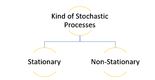
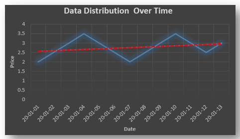
Stationary: A time series is said to be stationary when all the moments of its probability distribution i.e. mean, variance , covariance etc. are invariant over time. It becomes quite easy forecast data in this kind of situation as the hidden patterns are recognizable which make predictions easy.

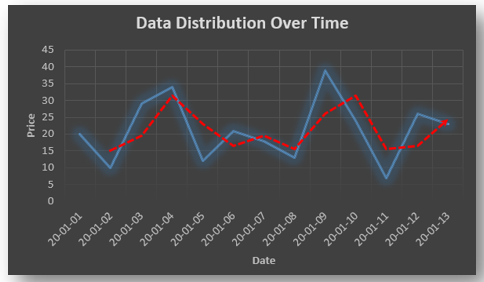
Non-stationary: A non-stationary time series will have a time varying mean or time varying variance or both, which makes it impossible to generalize the time series over other time periods.

Non stationary processes can further be explained with the help of a term called Random walk models. This term or theory usually is used in stock market which assumes that stock prices are independent of each other over time. Now there are two types of random walks:
Random walk with drift : When the observation that is to be predicted at a time ‘t’ is equal to last period’s value plus a constant or a drift (α) and the residual term (ε). It can be written as
Yt= α + Yt-1 + εt
The equation shows that Yt drifts upwards or downwards depending upon α being positive or negative and the mean and the variance also increases over time.
Random walk without drift: The random walk without a drift model observes that the values to be predicted at time ‘t’ is equal to last past period’s value plus a random shock.
Yt= Yt-1 + εt
Consider that the effect in one unit shock then the process started at some time 0 with a value of Y0
When t=1
Y1= Y0 + ε1
When t=2
Y2= Y1+ ε2= Y0 + ε1+ ε2
In general,
Yt= Y0+∑ εt
In this case as t increases the variance increases indefinitely whereas the mean value of Y is equal to its initial or starting value. Therefore the random walk model without drift is a non-stationary process.

So, with that we come to the end of the discussion on the Time Series. Hopefully it helped you understand time Series, for more information you can also watch the video tutorial attached down this blog. DexLab Analytics offers machine learning courses in delhi. To keep on learning more, follow DexLab Analytics blog.


.

Top 5 Industry Use Cases of Predictive Analytics

Top 5 Industry Use Cases of Predictive Analytics

Predictive analytics is an effective in-hand tool crafted for data scientists. Thanks to its quick computing and on-point forecasting abilities! Not only data scientists, but also insurance claim analysts, retail managers and healthcare professionals enjoy the perks of predictive analytics modeling – want to know how?

Below, we’ve enumerated a few real-life use cases, existing across industries, threaded with the power of data science and predictive analytics. Ask us, if you have any queries for your next data science project! Our data science courses in Delhi might be of some help.

Customer Retention

Losing customers is awful. For businesses. They have to gain new customers to make up for the loss in revenue. But, it can cost more, winning new customers is usually hailed more costly than retaining older ones.

Predictive analytics is the answer. It can prevent reduction in the customer base. How? By foretelling you the signs of customer dissatisfaction and identifying the customers that are most likely to leave. In this way, you would know how to keep your customers satisfied and content, and control revenue slip offs.

Customer Lifetime Value

Marketing a product is the crux of the matter. Identifying customers willing to spend a large part of their money, consistently for a long period of time is difficult to find. But once cracked, it helps companies optimize their marketing efforts and enhance their customer lifetime value.

2

Quality Control

Quality Control is significant. Over time, shoddy quality control measures will affect customer satisfaction ratio, purchasing behavior, thus impacting revenue generation and market share.

Further, low quality control results in more customer support expenses, repairs and warranty challenges and less systematic manufacturing. Predictive analytics help provide insights on potential quality issues, before they turn into crucial company growth hindrances.  

Risk Modeling

Risk can originate from a plethora of source, and it can be any form. Predictive analytics can address critical aspects of risk – it collects a huge number of data points from many organizations and sort through them to determine the potential areas of concern.

What’s more, the trends in the data hint towards unfavorable circumstances that might impact businesses and bottom line in an adverse way. A concoction of these analytics and a sound risk management approach is what companies truly need to quantify the risk challenges and devise a perfect course of action that’s indeed the need of the hour.

Sentiment Analysis

It’s impossible to be everywhere, especially when being online. Similarly, it’s very difficult to oversee everything that’s said about your company.

Nevertheless, if you amalgamate web search and a few crawling tools with customer feedback and posts, you’d be able to develop analytics that’d present you an overview of the organization’s reputation along with its key market demographics and more. Recommendation system helps!

All hail Predictive Analytics! Now, maneuver beyond fuss-free reactive operations and let predictive analytics help you plan for a successful future, evaluating newer areas of business scopes and capabilities.

Interested in data science certification? Look up to the experts at DexLab Analytics.

The blog has been sourced fromxmpro.com/10-predictive-analytics-use-cases-by-industry

Interested in a career in Data Analyst?

To learn more about Data Analyst with Advanced excel course – Enrol Now.
To learn more about Data Analyst with R Course – Enrol Now.
To learn more about Big Data Course – Enrol Now.

To learn more about Machine Learning Using Python and Spark – Enrol Now.
To learn more about Data Analyst with SAS Course – Enrol Now.
To learn more about Data Analyst with Apache Spark Course – Enrol Now.
To learn more about Data Analyst with Market Risk Analytics and Modelling Course – Enrol Now.

Predictive Analytics: The Key to Enhance the Process of Debt Collection

Predictive Analytics: The Key to Enhance the Process of Debt Collection

A wide array of industries has already engaged in some kind of predictive analytics – numerical analysis of debt collection is relatively a recent addition. Financial analysts are now found harnessing the power of predictive analytics to cull better results out for their clients, and measure the effectiveness of their strategies and collections.

Let’s see how predictive analytics is used in debt collection process:

2

Understanding Client Scoring (Risk Assessment)

Since the late 1980’s, FICO score is regarded as the golden standard for determining creditworthiness and loan application. But, however, machine learning, particularly predictive analytics can replace it, and develop an encompassing portrait of a client, taking into effect more than his mere credit history and present debts. It can also include his social media feeds and spending trajectory.

Evaluating Payment Patterns

The survival models evaluate each client’s probability of becoming a potential loss. If the account shows a continuous downward trend, then it should be regarded soon as a potential risk. Predictive analytics can help identify spending patterns, indicating the struggles of each client. A system can be developed which self-triggers whenever any unwanted pattern transpires. It could ask the client if they need any help or if they are going through a financial distress, so that it can help before the situation turns beyond repairs.

For R predictive modeling training courses, visit DexLab Analytics.

Cash Flow Predictions

Businesses are keen to know about future cash flows – what they can expect! Financial institutions are no different. Predictive analytics helps in making more appropriate predictions, especially when it comes to receivables.

Debt collector’s business models are subject to the ability to forecast the success of collection operations, and ascertaining results at the end of each month, before the billing cycle initiates. As a result, the workforce of the company is able to shift their focus from the potential payers to those who would not be able to meet their obligations. This shift in focus helps!

Better Client Relationship

Predictive analytics weave wonders; not only it has the ability to point which clients are the highest risks for your company, but also predict the best time to contact them to reap maximum results. What you need to do is just visit the logs of past conversations.

Challenges

Last, but not the least, all big data models face a common challenge – data cleaning. As it’s a process of wastage in and out, before starting with prediction, company should deal with this problem at first to construct a pipeline, for feeding in the data, clean it and use it for neural network training.

In a concluding statement, predictive analytics is the best bet for debt and revenue collection – it boosts conversion rates at the right time with the right people. If you want to study more about predictive analytics, and its varying uses in different segments of industry, enroll in R Predictive Modelling Certification training at DexLab Analytics. They provide superior knowledge-intensive training to interested individuals with added benefit of placement assistance. For more, visit their website.


The blog has been sourced fromdataconomy.com/2018/09/improving-debt-collection-with-predictive-models


Interested in a career in Data Analyst?

To learn more about Data Analyst with Advanced excel course – Enrol Now.
To learn more about Data Analyst with R Course – Enrol Now.
To learn more about Big Data Course – Enrol Now.

To learn more about Machine Learning Using Python and Spark – Enrol Now.
To learn more about Data Analyst with SAS Course – Enrol Now.
To learn more about Data Analyst with Apache Spark Course – Enrol Now.
To learn more about Data Analyst with Market Risk Analytics and Modelling Course – Enrol Now.

5 Best Tools Transforming Predictive Analytics in 2018

5 Best Tools Transforming Predictive Analytics in 2018

Gone are the days of sloppy decision-making techniques. Competitive businesses are embracing predictive analytics and associated tools.

Predictive analytics is a real game changer that allows companies to implement marketing strategies and serve customers with renewed efficiency. Customers in their natural interactions and networking with a company leave behind huge amounts of data. Predictive models extract valuable information from all this data, thereby helping enhance the performance of products and services, promoting better customer retention strategies, and improving core business competencies.

‘’The capacity for predictive analytics to learn from experience is what renders this technology effective, differentiating it from other business intelligence tools and analytics techniques’’, says the predictive analytics experts at Quantzig.

From thoroughly examining data, to figuring out correlations and patterns in data, predictive analytics tools effectively manage the entire business process. In this blog, we talk about some of the latest predictive analytics tools that are all the rage in 2018! So let’s dive in!

SAP Business Objects:

  • A powerful Business Intelligence platform that provides techniques to make swift and informed business decisions.
  • Offers a novel perspective on forming scalable solutions
  • SAP Business Object helps develop insights that encourage real time actions.
  • Enables users to visualize data in a self-serving manner

Image Source: Technosap

IBM Predictive Analytics:

  • Offers predictive analytics solutions that are simple to use and meet the requirements of different types of businesses.
  • Two important softwares, namely IBM SPSS Modeler and IBM SPSS Analytics, allow all users to implement predictive analytics and improve their businesses, irrespective of their skill levels.
  • The platform helps prevent frauds and maximizes profits.
  • It transforms extraneous data into predictive insights that steer key business decisions.
  • It is built with abilities to perform geospatial analysis and text analytics.
  • Runs on open source platforms with optional coding
  • Secure and private

Image Source: SlideShare

QlikView:

  • Flexible and easy-to-use business intelligence platform
  • Created by QlikTech
  • Allows enterprises to pull out relevant information from a given data set, which in turn helps design guided analytics applications.
  • Platform adopts a user-driven approach towards building charts and creating dashboards
  • BARC’ BI Survey 10 recognizes the ‘Agile BI’ ability of QlikView

Halo:

  • Ideal pick for an uninterrupted supply chain management system that aids in business forecasting
  • A smart platform with a dependable data repository, where cases can be run over and over again in order to perfectly match predictions with results.
  • Accessible through all kinds of browsers and available for cloud or hosted.
  • Self-serving nature of supply chain management allow organizations to increase customer satisfaction.

Image Source: Software Advice

Dataiku-DSS:

  • Dataiku is capable of transforming raw data into predictions.
  • Allows users to employ analytics appropriate algorithms
  • Allows users to leverage available libraries and apply custom codes in R and Python
  • Permits integration of external libraries by means of code API’s
  • Equipped with 80+ in-built functions that help investigate and clean raw forms of data
  • The best feature is a visual data profile at each step of analysis.

Image source: The Dataiku Blog

Want to learn SAS Predictive Modeling? Contact DexLab Analytics. The industry-experts at DexLab offer excellent SAS predictive modeling training. It encompasses theoretical understanding of core concepts and hands-on experience.


Interested in a career in Data Analyst?

To learn more about Data Analyst with Advanced excel course – Enrol Now.
To learn more about Data Analyst with R Course – Enrol Now.
To learn more about Big Data Course – Enrol Now.

To learn more about Machine Learning Using Python and Spark – Enrol Now.
To learn more about Data Analyst with SAS Course – Enrol Now.
To learn more about Data Analyst with Apache Spark Course – Enrol Now.
To learn more about Data Analyst with Market Risk Analytics and Modelling Course – Enrol Now.

The ABC of Summary Statistics and T Tests in SAS

The ABC of Summary Statistics and T Tests in SAS

Getting introduced to statistics for SAS training? Then, you must know how to create summary statistics (such as sample size, mean, and standard deviation) to test hypotheses and to figure confidence intervals. In this blog, we will show you how to furnish summary statistics (instead of raw data) to PROC TTEST in SAS, how to develop a data set that includes summary statistics and how to run PROC TTEST to calculate a two-sample or one-sample t test for the mean.

So, let’s start!

2

Running a two-sample t test for difference of means from summarized statistics

Instead of going the clichéd way, we will start with establishing a comparison between the mean heights of 19 students, based on gender – the data is held in the Sashelp class data set.

Observe the below SAS statements that sorts the data by the grouping variable, calling PROC MEANS and printing a subset of the statistics:

proc sort data=sashelp.class out=class; 
   by sex;                                /* sort by group variable */
run;
proc means data=class noprint;           /* compute summary statistics by group */
   by sex;                               /* group variable */
   var height;                           /* analysis variable */
   output out=SummaryStats;              /* write statistics to data set */
run;
proc print data=SummaryStats label noobs; 
   where _STAT_ in ("N", "MEAN", "STD");
   var Sex _STAT_ Height;
run;

summarystats1

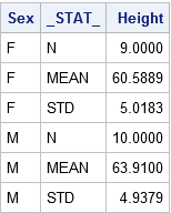
The table reflects the structure of the Summary Stats set for two sample tests. The two samples used here are differentiated on the levels of the Sex Variable (‘F’ for females and ‘M’ for males). The _STAT_ column shows the name of the statistic implemented here. The Height column depicts the value of the statistics for individual group.

Get SAS certification Delhi from DexLab Analytics today!

The problem: The heights of sixth-grade students are normally distributed. Random samples of n1=9 females and n2=10 males are selected. The mean height of the female sample is m1=60.5889 with a standard deviation of s1=5.0183. The mean height of the male sample is m2=63.9100 with a standard deviation of s2=4.9379. Is there evidence that the mean height of sixth-grade students depends on gender?

Here, you have to do nothing special to get the PROC TTEST – whenever the procedure gets the sight of the respective variable _STAT_ and any unique values, the procedure understands that the data set comprises summarized statistics. The following representation compares the mean heights of males and females:

proc ttest data=SummaryStats order=data
           alpha=0.05 test=diff sides=2; /* two-sided test of diff between group means */
   class sex;
   var height;
run;

summarystats1

Check the confidence intervals for the standard deviations and also that the output includes 95% confidence intervals for group means.

In the second table, the ‘Pooled’ row radiates out the impression that both the variances of two groups are more or less equal, which is somewhat true even. The value of the t statistic is t = -1.45 with a two-sided p-value of 0.1645.

The syntax for the PROC TTEST statement allows you to change the type of hypothesis test and the significance level. To support this, you can now run a one-sided test for the alternative hypothesis μ1 < μ2 at the 0.10 significance level just by using:

proc ttest ... alpha=0.10 test=diff sides=L;  /* Left-tailed test */

Running a one-sample t test of the mean from summarized statistics

In the above section, you have learnt to create the summary statistics from PROC MEANS. Nevertheless, you can also generate the summary statistic manually, if you lack original data.

The problem: A research study measured the pulse rates of 57 college men and found a mean pulse rate of 70.4211 beats per minute with a standard deviation of 9.9480 beats per minute. Researchers want to know if the mean pulse rate for all college men is different from the current standard of 72 beats per minute.

The following statements jots down the summary statistics for a data set, asks PROC TTEST to perform a one-sample test of the null hypothesis μ = 72 against a two-sided alternative hypothesis:

data SummaryStats;
  infile datalines dsd truncover;
  input _STAT_:$8. X;
datalines;
N, 57
MEAN, 70.4211
STD, 9.9480
;
 
proc ttest data=SummaryStats alpha=0.05 H0=72 sides=2; /* H0: mu=72 vs two-sided alternative */
   var X;
run;

summarystats3 (2)

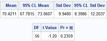
The outcome is a 95% confidence interval for the mean containing a value 72. The value of the t statistic is t = -1.20, which corresponds to a p-value of 0.2359. Therefore, the data fails in rejecting the null hypothesis at the 0.05 significance level.

For more informative blogs and news about SAS course, drop by our prime SAS predictive modeling training institute DexLab Analytics.

 
This post originally appeared onblogs.sas.com/content/iml/2017/07/03/summary-statistics-t-tests-sas.html
 

Interested in a career in Data Analyst?

To learn more about Data Analyst with Advanced excel course – Enrol Now.
To learn more about Data Analyst with R Course – Enrol Now.
To learn more about Big Data Course – Enrol Now.

To learn more about Machine Learning Using Python and Spark – Enrol Now.
To learn more about Data Analyst with SAS Course – Enrol Now.
To learn more about Data Analyst with Apache Spark Course – Enrol Now.
To learn more about Data Analyst with Market Risk Analytics and Modelling Course – Enrol Now.

How Predictive Analysis Could Have Saved the World from Ransomware

How Predictive Analysis Could Have Saved the World from Ransomware
 

Kudos to you, if you have stayed offline for the last couple of days, so you could actually spend the weekend well with your family and loved ones. The world is reeling under the shattering news surrounding WannaCry Ransomware this weekend. The situation was worse on Monday, after the offices opened. Going by the figures, revealed out on Monday evening by Elliptic, a Bitcoin forensics firm, which is keeping a watch overall – $57,282.23 in ransom has been shelled out to the hackers of Ransomware malware attack, who took over hundreds and thousands of computers worldwide on Friday and through the weekend.

Continue reading “How Predictive Analysis Could Have Saved the World from Ransomware”

Historians Make Use of Predictive Modeling

Predictive Modelling

Predictive modeling figures at the top of the list of new techniques put in to use by researchers in order to make out key archeological sites. The methodology used is not that complex. It makes predictions on the location of archeological sites having for its basis the qualities that are common to the sites already known. And the best news is that it works like a charm. A group of archeologists working in the company Logan Simpson which operates out of Utah discovered no less than 19 individual archeological sites containing many biface blades as well as stone points in addition to other artifacts that belong to the Paleoarchaic Period which ranges from 7,000 to 12,000 years ago.

2

The location of the site is about 160 km or 100 miles from Las Vegas, Nevada. The group of researchers also came across lakes and streams that disappeared long before. According to archeologists the sites were perhaps put into used by a number of groups of gatherers and hunters in the ancient times. The sites are scattered widely and also are scarce and could herald an understanding of the human activity that took place throughout the length and breadth of the Great Basin as a warmer climate prevailed after the end of the Ice Age. Their remoteness ensured that they remain unfound when traditional methods are employed.

How Predictive Analysis Could Have Saved the World from Ransomware – @Dexlabanalytics.

In Nevada’s Dry Lake Valley, Delamar Valley and Kane Springs archeologists have discovered sites like Clovis, Lake Mojave and also Silver Lake that contains some stone tools constructed according to styles prevalent as far as 12,000 years back.The project was funded by the Lincoln County Archeological Initiative from the Bureau of Land Management. It made use of GIS or geographic information system technology in order to make predictions about activity belonging to the Pleistocene-Holocene period.

 
Read Also: How Data Preparation Changed Post Predictive Analytics Model Implementation


The predictive modeling put into use took in to account the fact that the Great Basin was way more wet and cool at the end period of the Pleistocene than the climate prevalent today and in all probability had attracted the attention of gatherers and hunters for several centuries. The process of mapping with GIS and aerial pictures amongst others was followed by pinpointing and ranking the various locations that hold the most promise.

How Predictive Analysis Works With Data Mining – @Dexlabanalytics.

Apart from the Paleoarchaic era, artifacts belonging to relatively more recent periods in History were also found which bear out that the sites at the lakeside had been used over the course of several millennia.

But the most important discovery was the proof that that Predictive Modeling on the basis of GIS works well and should be included in the arsenal of tools of archeologists trying to discover prehistoric sites .

 
Read Also: Predictive Analytics: In conversation with Adam Bataran, Managing Director of GTM Global Salesforce Platforms at Bluewolf
 

Make predictive analytics your best friend for life and career with easy and comprehensive SAS training courses in Delhi by DexLab Analytics. For more information about this premier SAS training institute, log into their website.


Interested in a career in Data Analyst?

To learn more about Data Analyst with Advanced excel course – Enrol Now.
To learn more about Data Analyst with R Course – Enrol Now.
To learn more about Big Data Course – Enrol Now.

To learn more about Machine Learning Using Python and Spark – Enrol Now.
To learn more about Data Analyst with SAS Course – Enrol Now.
To learn more about Data Analyst with Apache Spark Course – Enrol Now.
To learn more about Data Analyst with Market Risk Analytics and Modelling Course – Enrol Now.

Call us to know more