Complete Guide to Credit Risk Modeling Techniques
A practical framework for PD, LGD, EAD and expected loss modeling in banking
Introduction
Between March 2018 and March 2021, gross non-performing assets at India’s public sector banks fell from a peak of 14.58% to 9.11% of advances. By September 2025, the system-wide gross NPA ratio for all scheduled commercial banks had dropped further, to a multi-decade low of 2.15%. That turnaround wasn’t accidental. Tighter underwriting, RBI’s Asset Quality Review, the Insolvency and Bankruptcy Code, and — underlying all of it — better credit risk models drove it.
The lesson for anyone building a career in banking analytics is straightforward. Credit risk is the single largest risk category banks carry on their balance sheets. How well a bank measures it directly determines capital adequacy, profitability, and long-term survival. A bank that underestimates default risk lends into losses it didn’t provision for. A bank that overestimates it prices good borrowers out of the market and loses share to competitors.
This guide walks through the complete framework professionals use to model credit risk. It covers the regulatory logic that makes credit risk modeling non-negotiable. It covers the three parameters that quantify it — PD, LGD, EAD. And it covers the statistical and machine learning techniques used to estimate each one. Maybe you’re a risk analyst preparing for an FRM exam. Maybe you’re a data scientist moving into banking analytics. Maybe you’re evaluating a credit risk modeling certification. Either way, this article builds the structured foundation technical interviews and real project work both expect.
By the end, you’ll understand the formulas. You’ll understand why each one exists, how professionals estimate it in practice, and where Indian banks apply it today.
What is Credit Risk and Why It Matters
Credit risk is the possibility that a borrower fails to meet a contractual debt obligation. The borrower could be an individual, a company, or a counterparty. Either way, it results in a financial loss for the lender. It is the risk that repayment doesn’t happen as agreed: a missed EMI, a defaulted corporate bond, a counterparty that can’t settle a derivative contract.
For a bank, credit risk isn’t one risk among many — it’s usually the dominant one. Loans and advances typically make up the largest share of a bank’s assets. Under the Basel framework, credit risk-weighted assets (RWA) form the biggest component of the capital a bank must hold. When credit risk is mismeasured, everything built on top of that measurement goes wrong too: capital adequacy ratios, loan pricing, provisioning, dividend capacity.
Why Credit Risk Modeling Matters to a Bank’s Survival
Three consequences flow directly from how well a bank models credit risk:
- Capital adequacy. Under Basel III, banks must hold capital proportional to the risk-weighted value of their assets. The Capital-to-Risk-Weighted-Assets Ratio (CRAR) for India’s scheduled commercial banks stood at a strong 17.2% as of September 2025 — well above the regulatory minimum. Risk measurement and provisioning discipline improved sharply after 2015, and it shows.
- Provisioning under IFRS 9. IFRS 9 replaced the incurred-loss model with an expected credit loss (ECL) model. Banks must now recognize losses before a default happens, based on modeled probabilities. That makes credit risk models a direct input into the profit and loss statement, not just a back-office risk tool.
- Pricing and portfolio strategy. A bank that can accurately rank borrowers by risk can price loans correctly, set appropriate limits, and choose which segments to grow or shrink. A bank that can’t ends up either losing good customers to competitors with sharper pricing, or accumulating bad loans that eventually show up as NPAs.
The RBI Regulatory Backdrop
The Reserve Bank of India has steadily tightened the credit risk framework banks operate under. Its 2015 Asset Quality Review forced transparent recognition of stressed assets that restructuring had previously hidden. More recently, in November 2023, the RBI raised risk weights on unsecured consumer credit — from 100% to 125% for banks. NBFC exposures saw a further increase. The goal: curb underpriced risk-taking in retail lending. The RBI has also begun articulating principle-based guidance for AI use in credit decisioning through its evolving regulatory framework. Model governance, not just model accuracy, is now squarely on the regulator’s radar.
This regulatory environment is precisely why credit risk modeling has become a core competency banks and NBFCs actively hire for — not an optional analytics add-on.
Core Components of Credit Risk Modeling
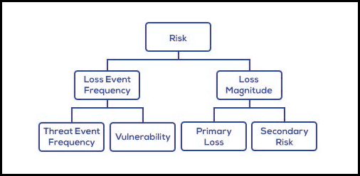
Every credit risk model, regardless of the statistical technique behind it, answers one question: how much money could the bank lose on this exposure, and how likely is that loss?
The industry-standard approach breaks “expected loss” into three independently modeled components:
1. Probability of Default (PD)
PD is the likelihood that a borrower will fail to meet their obligations within a defined time horizon. That’s typically 12 months for regulatory capital purposes, or lifetime PD under IFRS 9 for certain asset stages. PD is expressed as a percentage. A PD of 3% means a 3% chance of default within the horizon, based on the borrower’s characteristics.
2. Loss Given Default (LGD)
Default doesn’t always mean total loss. If a borrower defaults, the bank usually recovers something — through collateral liquidation, guarantees, or restructuring. LGD is the proportion of the exposure the bank expects to actually lose after recoveries. It’s expressed as a percentage of the exposure. An LGD of 40% means that, on average, the bank recovers 60% of what it’s owed after a default.
3. Exposure at Default (EAD)
EAD is the total value the bank carries at the moment of default — not the sanctioned limit, but the amount actually outstanding. For a term loan, this is close to the outstanding balance. Revolving facilities like credit cards or cash credit limits work differently. There, EAD must account for the possibility that the borrower draws down more of the limit before defaulting.
Putting It Together: Expected Loss
These three parameters combine into the foundational credit risk formula:
Expected Loss (EL) = PD × LGD × EAD
Consider a simple example: a bank has an outstanding exposure (EAD) of ₹1 crore to a borrower with a PD of 4% and an LGD of 45%.
Expected Loss = 0.04 × 0.45 × ₹1,00,00,000 = ₹1,80,000
This ₹1.8 lakh isn’t a one-off loss estimate for a single account. It’s the amount the bank should provision for, on average, across a portfolio of similar loans. Multiply this calculation across thousands of accounts, segmented by product, geography, and borrower type. The result is a portfolio-level expected loss figure that feeds directly into provisioning, pricing, and capital planning.
Why This Formula Is a Simplification
EL = PD × LGD × EAD is the standard, industry-wide formula — it’s not wrong. But it rests on an assumption worth naming explicitly: that PD, LGD, and EAD are independent of one another. In reality they aren’t. Recoveries tend to get worse exactly when default rates spike, because both track the same macroeconomic cycle. A recession depresses collateral values and pushes more borrowers into default at the same time. Multiplying three independent point estimates understates loss in exactly the scenarios that matter most. That’s why regulators require downturn LGD and downturn EAD/CCF add-ons rather than accepting benign-cycle averages.
From Single-Period EL to Lifetime ECL
The formula above is also a single-period number, typically 12 months. Under IFRS 9, lifetime ECL for Stage 2 and Stage 3 assets isn’t one multiplication. It’s a discounted sum of marginal expected losses across every remaining period of the loan’s life:
Lifetime ECL = Σₜ (marginal PDₜ × LGDₜ × EADₜ) × discount factorₜ
That distinction matters in practice. A 12-month EL figure and a lifetime ECL figure for the same loan can differ substantially. Conflating the two is a common — and consequential — modeling error.
Each of the three components — probability of default, loss given default, and EAD — demands its own data, statistical techniques, and validation standards. Getting the overall expected loss number right depends entirely on getting each of these three right individually. It also depends on staying honest about where the simplifying assumptions break down.
Probability of Default (PD) Estimation
PD estimation is where most credit risk modeling careers begin, because it has the richest data history and the most mature statistical toolkit.
The Data Foundation
PD models draw on historical loan performance data: borrower demographics, financial ratios, repayment history, bureau scores (like CIBIL in India), and macroeconomic variables. The target variable is binary. Did the borrower default within the observation window, typically defined as 90 days past due (DPD), or not?
Method 1: Logistic Regression
Logistic regression remains the industry workhorse for PD modeling, and for good reason. It’s interpretable, regulator-friendly, and produces a probability output directly — exactly what PD requires.
The logistic regression model estimates:
PD = 1 / (1 + e^-(β₀ + β₁X₁ + β₂X₂ + … + βₙXₙ))
X₁ through Xₙ are borrower characteristics: debt-to-income ratio, bureau score, vintage, loan-to-value ratio, and so on. Analysts estimate the β coefficients from historical default data.
Worked example: Suppose a simplified model uses two variables — bureau score and debt-to-income (DTI) ratio — and produces this equation:
Logit(PD) = -3.5 + (-0.02 × Bureau Score) + (2.1 × DTI)
For a borrower with a bureau score of 720 and a DTI of 0.35:
Logit(PD) = -3.5 + (-0.02 × 720) + (2.1 × 0.35) = -3.5 − 14.4 + 0.735 = -17.165
PD = 1 / (1 + e^17.165) ≈ 0.00003, or effectively near-zero risk — consistent with a strong bureau score and moderate leverage.
In practice, banks convert these raw PD outputs into a credit scorecard. It’s a points-based system: each variable band — score range, income bracket, tenure — contributes points that sum to a final score. That score maps back to a PD and a risk grade, AAA to D for instance. Most retail lending decision engines run on exactly this system.
Method 2: Survival Analysis
Logistic regression answers “will this borrower default within 12 months?” It doesn’t naturally answer “when.” Survival analysis models the time to default instead, using techniques like the Cox Proportional Hazards model or Kaplan-Meier estimation. It treats default as an “event.” It treats non-defaulted, still-active loans as “censored” observations.
This matters for two practical reasons. First, it lets banks estimate lifetime PD curves, which IFRS 9 requires for Stage 2 and Stage 3 assets. Second, it naturally handles loans that are still performing at the end of the observation period. It doesn’t treat them as “non-defaults” the way a simple logistic model would. That subtlety matters a great deal in mortgage and long-tenure corporate lending portfolios.
Machine Learning Extensions
Random forests, gradient boosting (XGBoost, LightGBM), and neural networks increasingly supplement — not always replace — logistic regression. This works particularly well where alternative data is available: transaction behavior, digital footprint, utility payment history. Industry research on large Indian banks backs this up. ML models can improve default prediction accuracy over ratio-based or bureau-only assessments, particularly for thin-file borrowers without a long credit history. The trade-off is interpretability. Regulators and internal model validation teams expect PD models to be explainable. That’s why techniques like SHAP (SHapley Additive exPlanations) have become standard for justifying ML-based PD outputs to auditors and regulators.
Common Mistakes in PD Modeling
- Treating bureau score as a sufficient standalone predictor without controlling for portfolio-specific behavior
- Ignoring population stability — a PD model trained on pre-pandemic data can be badly miscalibrated for a post-pandemic portfolio
- Failing to account for right-censoring when using a fixed observation window
- Overfitting on a small default sample, which is common in low-default portfolios like corporate or sovereign lending
Loss Given Default (LGD) and Recovery
PD tells you whether a loss will happen. LGD tells you how big it will be once it does. Most practitioners consider it the harder of the two to model well. Default events are relatively rare, and recovery processes can take years to conclude.
What Drives LGD
LGD is shaped primarily by three factors:
- Collateral coverage and quality. A secured home loan with a well-documented, liquid property as collateral typically carries a far lower LGD than an unsecured personal loan. The reason: the bank has a tangible asset to recover value from.
- Seniority of claim. In corporate lending, senior secured lenders recover more than subordinated or unsecured creditors in a resolution or liquidation.
- Recovery mechanism and timeline. In India, recovery routes include SARFAESI Act enforcement, Debt Recovery Tribunals, and the Insolvency and Bankruptcy Code (IBC). These matter enormously for LGD estimation. IBC-driven recoveries have averaged around 94% of the fair value of resolved businesses, though considerably less against the original claim amount. System-wide NPA recovery rates for scheduled commercial banks have roughly doubled, from 13.2% in FY18 to 26.2% in FY25, reflecting stronger legal recovery infrastructure.
The Recovery Rate Relationship
LGD and recovery rate are two sides of the same coin:
LGD = 1 − Recovery Rate
That relationship is correct. But it’s easy to misapply, because “recovery rate” is doing a lot of work in that equation. It has to mean the economic recovery rate: the present value of net recoveries, after two adjustments. First, discount every recovered cash flow back to the default date, to account for the time value of money. Second, subtract the direct and indirect costs of recovery — legal fees, collateral liquidation costs, workout team overhead. A workout can take two to three years in India, even under IBC timelines. A rupee recovered in year three is worth meaningfully less than a rupee recovered on day one.
The common mistake: using the nominal recovery rate instead. That’s raw cash eventually recovered, divided by exposure, with no discounting and no cost deduction. It overstates the recovery rate and, by direct consequence, understates LGD. Say a bank nominally recovers 65% of exposure post-default, but that recovery arrives over three years and costs 8% of exposure in legal and liquidation expenses. The economic recovery rate falls well below 65%. The resulting LGD lands correspondingly higher than the naive “35%” the nominal figure would suggest.
Collateral Valuation
For secured lending, LGD modeling starts with realistic collateral valuation — not the value at origination, but the expected value at the time of liquidation, discounted for:
- Market depreciation of the asset class (property, equipment, vehicles)
- Haircut for forced-sale conditions versus fair market value
- Time-to-recovery, since a three-year legal process erodes present value even if the nominal recovery is high
- Direct recovery costs (legal fees, auctioneer fees, administrative costs)
Statistical Methods for LGD
- Workout LGD (the standard approach): Banks track every actual default in their historical data. They record all cash flows recovered post-default: collateral sale proceeds, settlement payments, guarantee invocations. Then they discount those cash flows back to the default date, using an appropriate discount rate, and net off recovery costs. This produces an empirical, account-level LGD. Analysts then average and segment it by product, collateral type, and vintage.
- Regression-based LGD models: Raw workout LGD is bounded between 0 and 1. It can occasionally exceed 1, when recovery costs surpass recoveries. Banks often use techniques suited to bounded outcomes instead. One option is beta regression. Another is a two-stage model: first predict whether any recovery occurs at all, then model the recovery amount conditional on recovery happening.
- Downturn LGD: Basel requires banks to estimate LGD under economic downturn conditions, not just average conditions, because collateral values and recovery rates both tend to fall exactly when default rates rise. This is a critical, frequently underestimated requirement. An LGD model calibrated only on benign-cycle data will understate loss severity in a stress scenario.
A Practical Note on LGD in Indian Retail Lending
For Indian home loans, LGD modeling relies heavily on loan-to-value (LTV) ratio at origination and current LTV, adjusted for property price movements. Property is the dominant recovery source here. Unsecured personal loans and credit cards work differently — they carry substantially higher and more volatile LGD, since recovery depends almost entirely on borrower cooperation, collection agency effectiveness, or write-off. That’s part of why the RBI’s 2023 risk-weight increase on unsecured credit targeted loss severity concerns explicitly.
<h2id=”exposure-at-default”>Exposure at Default (EAD) Calculation
EAD often gets treated as the “simple” component of the PD × LGD × EAD formula, but any product with a revolving or undrawn component needs its own careful modeling.
Why EAD Isn’t Just the Current Balance
For a fully drawn term loan, EAD is straightforward. It stays close to the outstanding principal balance at any point in time, adjusted for scheduled amortization. Products like credit cards, overdrafts, and cash credit facilities work differently. A borrower can draw down additional funds between the assessment date and the moment of default. A borrower approaching financial distress often draws their credit line closer to the limit right before defaulting. That means EAD tends to run higher than the current outstanding balance, for exactly the accounts where it matters most.
The Credit Conversion Factor (CCF)
To capture this, banks use the Credit Conversion Factor (CCF) — the proportion of the currently undrawn commitment they expect to see drawn down before default.
EAD = Current Outstanding Balance + (CCF × Undrawn Commitment)
Worked example: A borrower has a credit card with a sanctioned limit of ₹5,00,000. The current outstanding balance is ₹2,00,000, leaving an undrawn commitment of ₹3,00,000. Historical data shows that, on average, borrowers who eventually default draw down 60% of their remaining undrawn limit before the default event (CCF = 0.60).
EAD = ₹2,00,000 + (0.60 × ₹3,00,000) = ₹2,00,000 + ₹1,80,000 = ₹3,80,000
This runs meaningfully higher than the ₹2,00,000 current balance. The expected loss calculation should use the ₹3,80,000 figure, not the current balance.
How CCF Is Estimated
Banks typically estimate CCF empirically, using a cohort approach. They identify accounts that defaulted. They look back at each account’s utilization level 12 months before default. Then they measure how much of the then-undrawn limit got drawn down by the time of default. Averaging this ratio across the portfolio — segmented by product type and current utilization band — produces the CCF estimates that feed EAD models.
CCF runs highest for revolving retail products like credit cards and overdrafts. It runs near-zero for term loans with no undrawn component. Corporate revolving credit facilities and working capital limits also require dedicated CCF modeling. Distressed corporate borrowers frequently draw down committed but unused credit lines as a liquidity buffer before default becomes evident.
EAD Under Basel and IFRS 9
Under the Basel Internal Ratings-Based (IRB) approach, EAD estimation follows the same downturn-conditioning logic as LGD. CCFs should reflect what happens under stressed conditions, since utilization tends to spike precisely when the broader environment deteriorates. Under IFRS 9, EAD projections also need to extend across the lifetime of the facility for Stage 2 and Stage 3 exposures, not just a fixed 12-month window.
Real-World Implementation in Banking
The theory behind PD, LGD, and EAD only matters if it translates into disciplined implementation. India’s banking sector over the past decade offers a clear illustration of what that looks like at scale.
The Turnaround in Numbers
Following the RBI’s 2015 Asset Quality Review, public sector banks’ gross NPA ratio rose sharply, as transparent recognition brought hidden stress to light. It peaked at 14.58% in March 2018. What followed was a sustained, model-driven cleanup. Recapitalization, tighter underwriting standards, and the Insolvency and Bankruptcy Code combined to bring the PSB gross NPA ratio down to 9.11% by March 2021, and further to 2.58% by March 2025. System-wide, across all scheduled commercial banks, the gross NPA ratio reached a multi-decade low of around 1.8%–2.15% through late 2025 and into 2026, per the RBI’s Financial Stability Report.
At the institution level, this shows up clearly in individual bank results. For the quarter ended March 2026, State Bank of India — India’s largest lender — reported a gross NPA ratio of 1.49% and a net NPA ratio of 0.39%. HDFC Bank reported a gross NPA ratio of 1.15% and net NPA ratio of 0.38%. These aren’t accidents of a benign credit cycle alone. They reflect years of investment: early warning systems, scorecard-based underwriting, stressed-asset monitoring infrastructure.
What Changed Operationally
Three implementation shifts are consistently cited across the sector:
- Early Warning Systems (EWS). Public sector banks have rolled out automated EWS frameworks with roughly 80 distinct triggers. These pull in third-party data to flag stress in borrowing accounts before they slip into NPA status. This shifts credit risk management from reactive classification to proactive monitoring.
- Machine learning-augmented scorecards. Industry research examining major Indian banks — SBI, HDFC, ICICI, Kotak Mahindra — found that machine learning techniques consistently outperform pure ratio-based or bureau-score-only assessments. The winning combination: logistic regression alongside random forests and neural networks, incorporating alternative data like transaction behavior and digital usage patterns. It works especially well for borrowers with thin credit files.
- Faster, more granular underwriting. The same research found loan approval times at many Indian banks have compressed, from several days to a matter of minutes for eligible segments. Automated, model-based decisioning drives this, rather than manual file review. That shift only became possible once PD and exposure models earned enough validated trust to run with minimal manual override.
The Governance Layer
None of this works without governance. The RBI’s ongoing regulatory review — including its recently articulated principle-based framework for AI use in banking — signals something important. As banks lean further into ML-driven credit risk models, model validation, explainability, and monitoring will matter as much as raw predictive accuracy. A model that can’t be explained to an auditor or regulator can’t be deployed at scale in a regulated balance sheet, no matter how well it performs statistically.
Interview Questions to Test Your Understanding
- Write out the expected loss formula and explain what each component represents.
- Why is logistic regression still preferred over more complex ML models for regulatory PD models?
- What’s the difference between workout LGD and downturn LGD, and why does Basel require the latter?
- Explain why EAD for a credit card is typically higher than the current outstanding balance.
- How would you validate a PD model’s performance? (Hint: think Gini coefficient, KS statistic, and calibration testing.)
Summary
Credit risk modeling breaks down a complex question: how much could a bank lose, and how likely is it? It splits that question into three independently estimated, rigorously validated components — Probability of Default, Loss Given Default, and Exposure at Default — combined through EL = PD × LGD × EAD. Analysts typically estimate PD through logistic regression and survival analysis, increasingly supplemented by explainable machine learning. LGD depends on collateral quality, recovery mechanisms, and downturn conditions. EAD requires modeling credit conversion factors for any revolving exposure. Together, these three parameters drive capital adequacy, IFRS 9 provisioning, and loan pricing. India’s banking sector’s asset quality turnaround over the past decade proves the point: disciplined credit risk modeling delivers at scale.
Frequently Asked Questions
Q1. What is the difference between credit risk and credit risk modeling?
Credit risk is the underlying possibility of borrower default. Credit risk modeling is the quantitative discipline of measuring that risk. It uses statistical and machine learning techniques to estimate PD, LGD, and EAD, so a bank can price, provision for, and manage the risk.
Q2. Is credit risk modeling the same as credit scoring?
Credit scoring is a subset of credit risk modeling, focused specifically on PD estimation for underwriting decisions. Full credit risk modeling also covers LGD, EAD, portfolio-level expected loss, stress testing, and regulatory capital calculation.
Q3. Which technique is better for PD modeling: logistic regression or machine learning?
Neither wins universally. Logistic regression remains preferred for regulatory capital models, thanks to its interpretability and regulator familiarity. Machine learning models can improve accuracy, particularly with alternative data. But they require additional explainability tooling — like SHAP — to meet governance and audit requirements.
Q4. What skills do I need to build a career in credit risk modeling?
You need statistics (logistic regression, survival analysis), proficiency in Python or SAS, familiarity with Basel and IFRS 9, and hands-on exposure to real credit datasets. Structured training that pairs regulatory context with practical model-building is generally the fastest path in.
Q5. How is credit risk modeling connected to IFRS 9?
IFRS 9 requires banks to recognize expected credit losses using forward-looking PD, LGD, and EAD estimates, rather than waiting for an actual default. Stage 1 assets use a 12-month figure, close to the standard EL = PD × LGD × EAD calculation. Stage 2 and 3 assets use lifetime ECL instead — a discounted sum of marginal expected losses across the loan’s remaining life, not a single multiplication.
Ready to Build These Skills Hands-On?
Understanding the theory behind PD, LGD, and EAD is the first step. Building bankable, interview-ready models — in Python or SAS, on real credit datasets, aligned to Basel and IFRS 9 — is what actually moves a career forward.
Explore Dexlab Analytics’ Credit Risk Modeling certification program to build PD, LGD, and EAD models from scratch, work through IFRS 9 ECL frameworks, and learn model validation techniques used by practicing risk teams.
.