In our previous blog we discussed about few of the basic functions of MQL like .find() , .count() , .pretty() etc. and in this blog we will continue to do the same. At the end of the blog there is a quiz for you to solve, feel free to test your knowledge and wisdom you have gained so far.
Given below is the list of functions that can be used for data wrangling:-
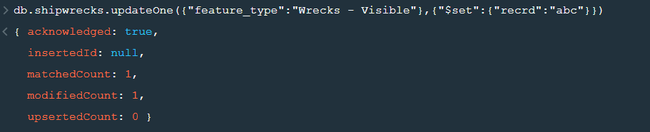
updateOne() :- This function is used to change the current value of a field in a single document.
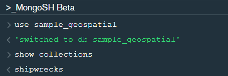
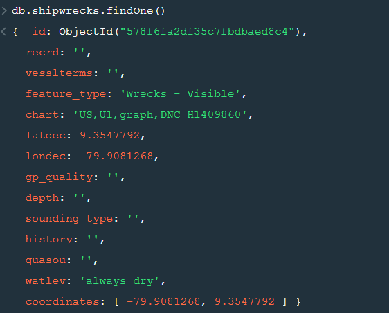
After changing the database to “sample_geospatial” we want to see what the document looks like? So for that we will use .findOne() function.
Now lets update the field value of “recrd” from ‘ ’ to “abc” where the “feature_type” is ‘Wrecks-Visible’.
Now within the .updateOne() funtion any thing in the first part of { } is the condition on the basis of which we want to update the given document and the second part is the changes which we want to make. Here we are saying that set the value as “abc” in the “recrd” field . In case you wanted to increase the value by a certain number ( assuming that the value is integer or float) you can use “$inc” instead.
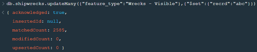
2. updateMany() :- This function updates many documents at once based on the condition provided.
3. deleteOne() & deleteMany() :- These functions are used to delete one or many documents based on the given condition or field.
4. Logical Operators :-
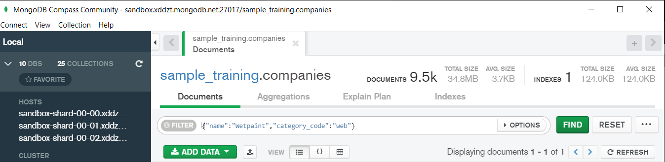
“$and” : It is used to match all the conditions.
“$or” : It is used to match any of the conditions.
The first code matches both the conditions i.e. name should be “Wetpaint” and “category_code” should be “web”, whereas the second code matches any one of the conditions i.e. either name should be “Wetpaint” or “Facebook”. Try these codes and see the difference by yourself.
So, with that we come to the end of the discussion on the MongoDB Basics. Hopefully it helped you understand the topic, for more information you can also watch the video tutorial attached down this blog. The blog is designed and prepared by Niharika Rai, Analytics Consultant, DexLab AnalyticsDexLab Analytics offers machine learning courses in Gurgaon. To keep on learning more, follow DexLab Analytics blog.
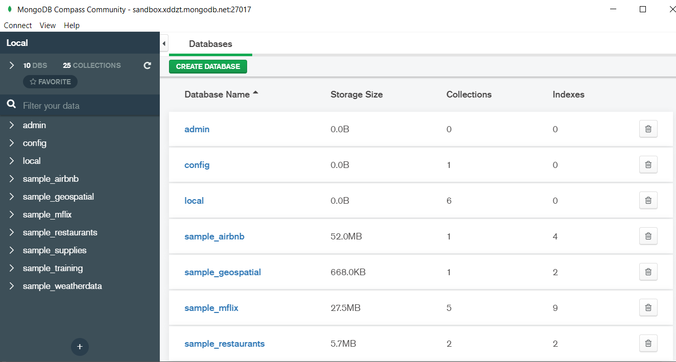
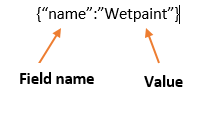
MongoDB is a document based database program which was developed by MongoDB Inc. and is licensed under server side public license (SSPL). It can be used across platforms and is a non-relational database also known as NoSQL, where NoSQL means that the data is not stored in the conventional tabular format and is used for unstructured data as compared to SQL and that is the major difference between NoSQL and SQL. MongoDB stores document in JSON or BSON format. JSON also known as JavaScript Object notation is a format where data is stored in a key value pair or array format which is readable for a normal human being whereas BSON is nothing but the JSON file encoded in the binary format which is quite hard for a human being to understand. Structure of MongoDB which uses a query language MQL(Mongodb query language):- Databases:- Databases is a group of collections. Collections:- Collection is a group fields. Fields:- Fields are nothing but key value pairs Just for an example look at the image given below:-
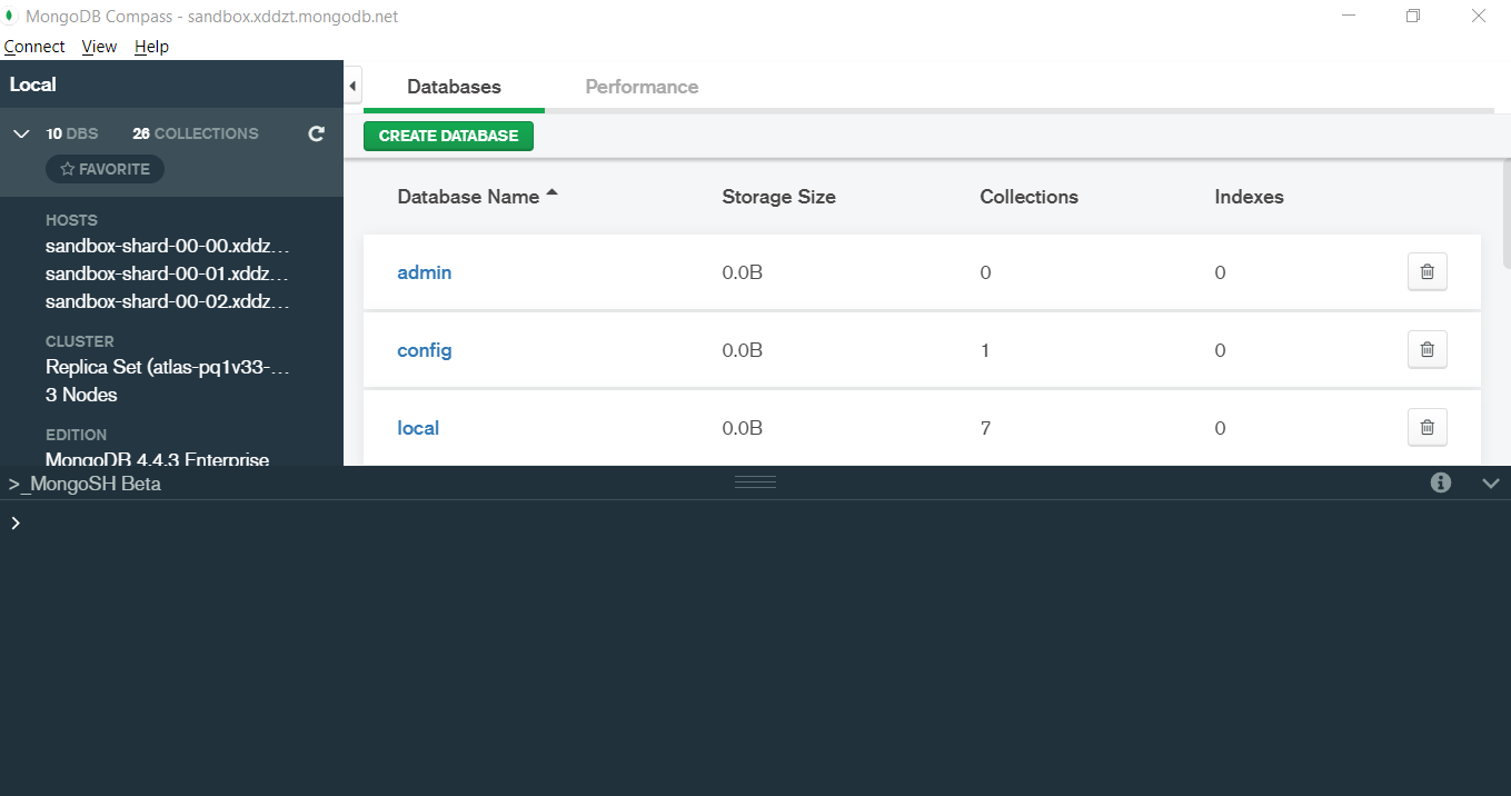
Here I am using MongoDB Compass a tool to connect to Atlas which is a cloud based platform which can help us write our queries and start performing all sort of data extraction and deployment techniques. You can download MongoDB Compass via the given link https://www.mongodb.com/try/download/compass
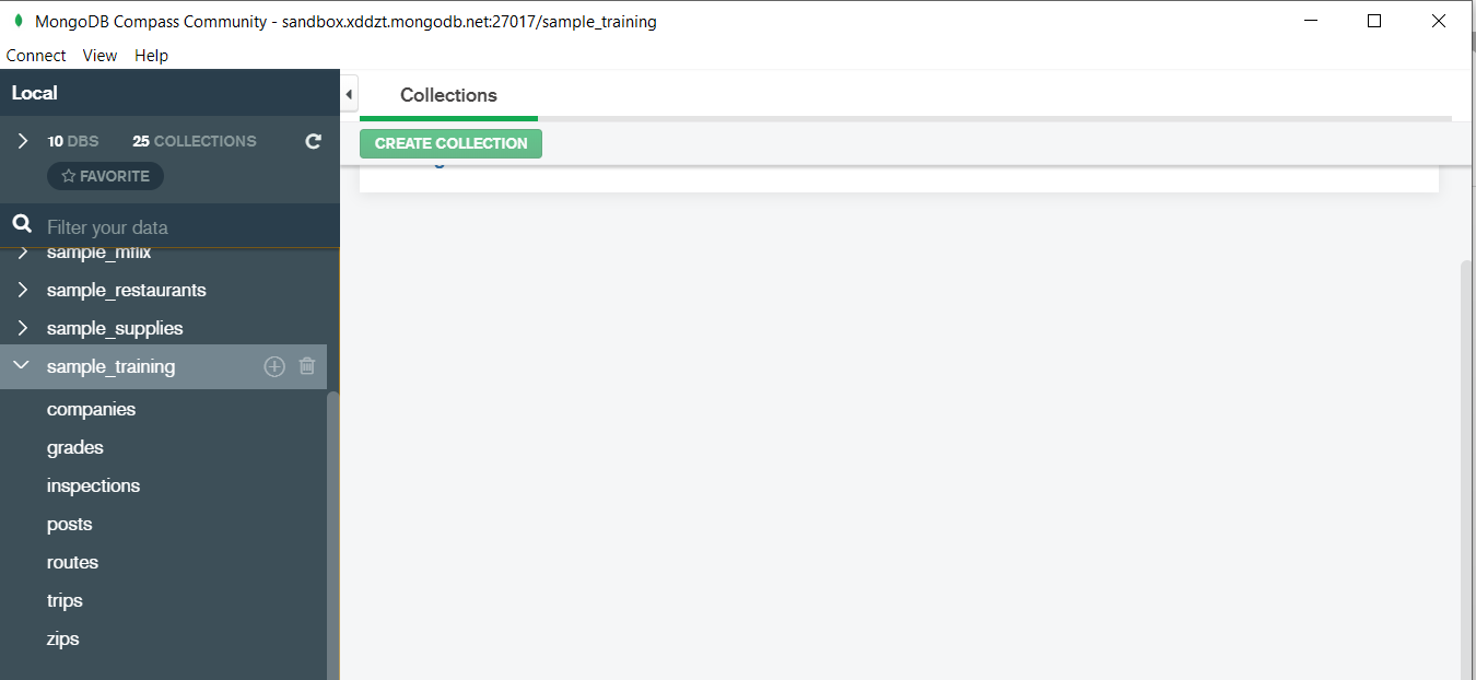
In the above image in the red box we have our databases and if we click on the “sample_training” database we will see a list of collections similar to the tables in sql.
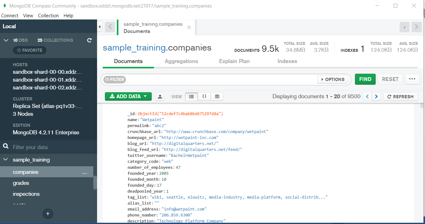
Now lets write our first query and see what data in “companies” collection looks like but before that select the “companies” collection.
Now in our filter cell we can write the following query:-
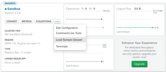
In the above query “name” and “category_code” are the key values also known as fields and “Wetpaint” and “web” are the pair values on the basis of which we want to filter the data. What is cluster and how to create it on Atlas? MongoDB cluster also know as sharded cluster is created where each collection is divided into shards (small portions of the original data) which is a replica set of the original collection. In case you want to use Atlas there is an unpaid version available with approximately 512 mb space which is free to use. There is a pre-existing cluster in MongoDB named Sandbox , which currently I am using and you can use it too by following the given steps:- 1. Create a free account or sign in using your Google account on https://www.mongodb.com/cloud/atlas/lp/try2-in?utm_source=google&utm_campaign=gs_apac_india_search_brand_atlas_desktop&utm_term=mongodb%20atlas&utm_medium=cpc_paid_search&utm_ad=e&utm_ad_campaign_id=6501677905&gclid=CjwKCAiAr6-ABhAfEiwADO4sfaMDS6YRyBKaciG97RoCgBimOEq9jU2E5N4Jc4ErkuJXYcVpPd47-xoCkL8QAvD_BwE 2. Click on “Create an Organization”. 3. Write the organization name “MDBU”. 4. Click on “Create Organization”. 5. Click on “New Project”. 6. Name your project M001 and click “Next”. 7. Click on “Build a Cluster”. 8. Click on “Create a Cluster” an option under which free is written. 9. Click on the region closest to you and at the bottom change the name of the cluster to “Sandbox”. 10. Now click on connect and click on “Allow access from anywhere”. 11. Create a Database User and then click on “Create Database User”. username: m001-student password: m001-mongodb-basics 12. Click on “Close” and now load your sample as given below :
Loading may take a while…. 13. Click on collections once the sample is loaded and now you can start using the filter option in a similar way as in MongoDB Compass In my next blog I’ll be sharing with you how to connect Atlas with MongoDB Compass and we will also learn few ways in which we can write query using MQL.
So, with that we come to the end of the discussion on the MongoDB. Hopefully it helped you understand the topic, for more information you can also watch the video tutorial attached down this blog. The blog is designed and prepared by Niharika Rai, Analytics Consultant, DexLab AnalyticsDexLab Analytics offers machine learning courses in Gurgaon. To keep on learning more, follow DexLab Analytics blog.
In this particular blog we will discuss about few of the basic functions of MQL (MongoDB Query Language) and we will also see how to use them? We will be using MongoDB Compass shell (MongoSH Beta) which is available in the latest version of MongoDB Compass.
Connect your Atlas cluster to your MongoDB Compass to get started. Latest version of MongoDB Compass will have this shell, so if you don’t find this shell then please install the latest version for this to work.
Now lets start with the functions.
find() :- You need this function for data extraction in the shell.
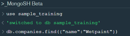
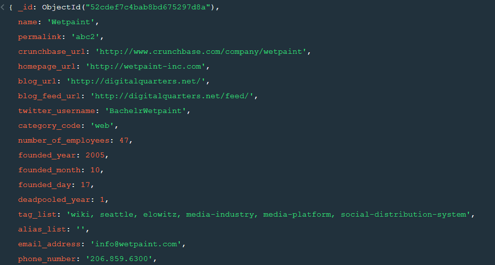
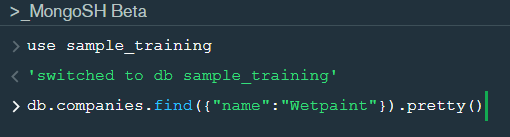
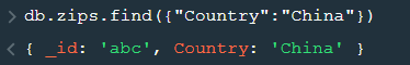
In the shell we need to first write the “use database name” code to access the database then use .find() to extract data which has name “Wetpaint”
For the above query we get the following result:-
The above result brings us to another function .pretty() .
2. pretty() :- this function helps us see the result more clearly.
Try it yourself to compare the results.
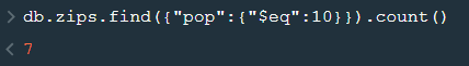
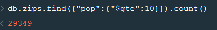
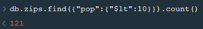
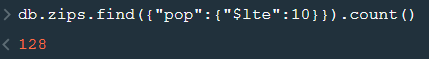
3. count() :- Now lets see how many entries we have by the company name “Wetpaint”.
So we have only one document.
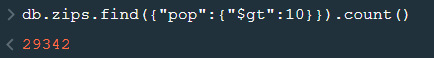
4. Comparison operators :-
“$eq” : Equal to
“$neq”: Not equal to
“$gt”: Greater than
“$gte”: Greater than equal to
“$lt”: Less than
“$lte”: Less than equal to
Lets see how this works.
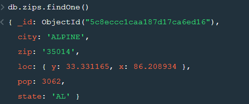
5. findOne() :- To get a single document from a collection we use this function.
6. insert() :- This is used to insert documents in a collection.
Now lets check if we have been able to insert this document or not.
Notice that a unique id has been added to the document by default. The given id has to be unique or else there will be an error. To provide a user defined id use “_id”.
So, with that we come to the end of the discussion on the MongoDB. Hopefully it helped you understand the topic, for more information you can also watch the video tutorial attached down this blog. The blog is designed and prepared by Niharika Rai, Analytics Consultant, DexLab AnalyticsDexLab Analytics offers machine learning courses in Gurgaon. To keep on learning more, follow DexLab Analytics blog.
This is another blog added to the series of time series forecasting. In this particular blog I will be discussing about the basic concepts of ARIMA model.
So what is ARIMA?
ARIMA also known as Autoregressive Integrated Moving Average is a time series forecasting model that helps us predict the future values on the basis of the past values. This model predicts the future values on the basis of the data’s own lags and its lagged errors.
When a data does not reflect any seasonal changes and plus it does not have a pattern of random white noise or residual then an ARIMA model can be used for forecasting.
There are three parameters attributed to an ARIMA model p, q and d :-
p :- corresponds to the autoregressive part
q:- corresponds to the moving average part.
d:- corresponds to number of differencing required to make the data stationary.
In our previous blog we have already discussed in detail what is p and q but what we haven’t discussed is what is d and what is the meaning of differencing (a term missing in ARMA model).
Since AR is a linear regression model and works best when the independent variables are not correlated, differencing can be used to make the model stationary which is subtracting the previous value from the current value so that the prediction of any further values can be stabilized . In case the model is already stationary the value of d=0. Therefore “differencing is the minimum number of deductions required to make the model stationary”. The order of d depends on exactly when your model becomes stationary i.e. in case the autocorrelation is positive over 10 lags then we can do further differencing otherwise in case autocorrelation is very negative at the first lag then we have an over-differenced series.
The formula for the ARIMA model would be:-
To check if ARIMA model is suited for our dataset i.e. to check the stationary of the data we will apply Dickey Fuller test and depending on the results we will using differencing.
In my next blog I will be discussing about how to perform time series forecasting using ARIMA model manually and what is Dickey Fuller test and how to apply that, so just keep on following us for more.
So, with that we come to the end of the discussion on the ARIMA Model. Hopefully it helped you understand the topic, for more information you can also watch the video tutorial attached down this blog. The blog is designed and prepared by Niharika Rai, Analytics Consultant, DexLab AnalyticsDexLab Analytics offers machine learning courses in Gurgaon. To keep on learning more, follow DexLab Analytics blog.
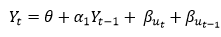
ARMA(p,q) model in time series forecasting is a combination of Autoregressive Process also known as AR Process and Moving Average (MA) Process where p corresponds to the autoregressive part and q corresponds to the moving average part.
Autoregressive Process (AR) :- When the value of Yt in a time series data is regressed over its own past value then it is called an autoregressive process where p is the order of lag into consideration.
Where,
Yt = observation which we need to find out.
α1= parameter of an autoregressive model
Yt-1= observation in the previous period
ut= error term
The equation above follows the first order of autoregressive process or AR(1) and the value of p is 1. Hence the value of Yt in the period ‘t’ depends upon its previous year value and a random term.
Moving Average (MA) Process :- When the value of Yt of order q in a time series data depends on the weighted sum of current and the q recent errors i.e. a linear combination of error terms then it is called a moving average process which can be written as :-
yt = observation which we need to find out
α= constant term
βut-q= error over the period q .
ARMA (Autoregressive Moving Average) Process :-
The above equation shows that value of Y in time period ‘t’ can be derived by taking into consideration the order of lag p which in the above case is 1 i.e. previous year’s observation and the weighted average of the error term over a period of time q which in case of the above equation is 1.
How to decide the value of p and q?
Two of the most important methods to obtain the best possible values of p and q are ACF and PACF plots.
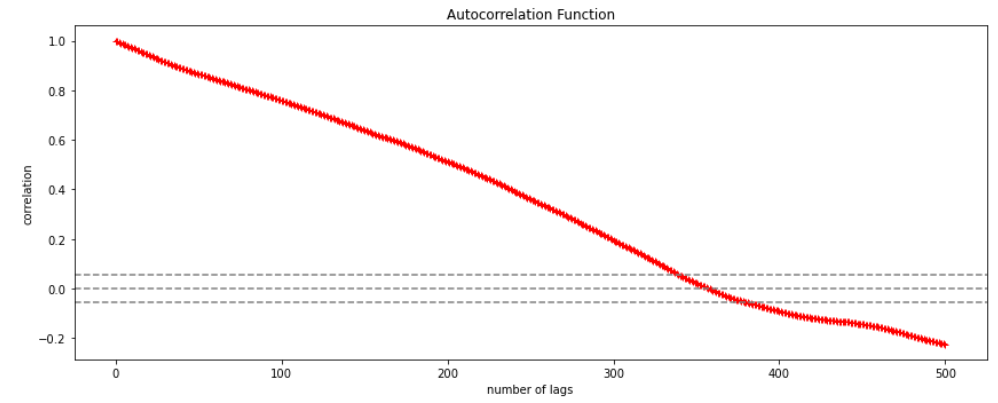
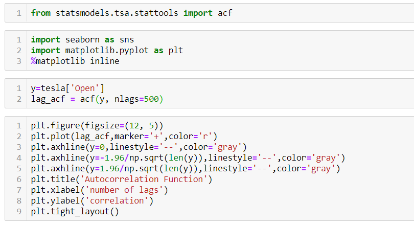
ACF (Auto-correlation function) :- This function calculates the auto-correlation of the complete data on the basis of lagged values which when plotted helps us choose the value of q that is to be considered to find the value of Yt. In simple words how many years residual can help us predict the value of Yt can obtained with the help of ACF, if the value of correlation is above a certain point then that amount of lagged values can be used to predict Yt.
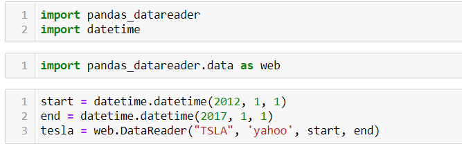
Using the stock price of tesla between the years 2012 and 2017 we can use the .acf() method in python to obtain the value of p.
.DataReader() method is used to extract the data from web.
The above graph shows that beyond the lag 350 the correlation moved towards 0 and then negative.
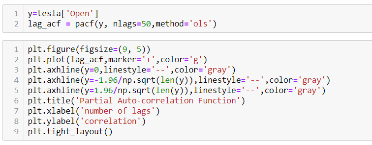
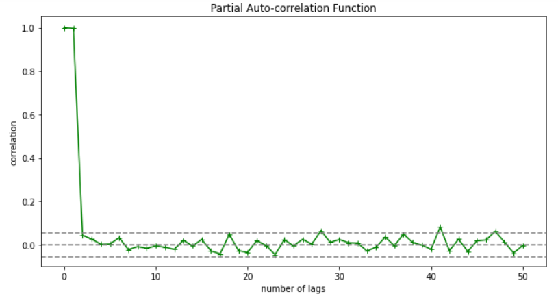
PACF (Partial auto-correlation function) :- Pacf helps find the direct effect of the past lag by removing the residual effect of the lags in between. Pacf helps in obtaining the value of AR where as acf helps in obtaining the value of MA i.e. q. Both the methods together can be use find the optimum value of p and q in a time series data set.
Lets check out how to apply pacf in python.
As you can see in the above graph after the second lag the line moved within the confidence band therefore the value of p will be 2.
So, with that we come to the end of the discussion on the ARMA Model. Hopefully it helped you understand the topic, for more information you can also watch the video tutorial attached down this blog. The blog is designed and prepared by Niharika Rai, Analytics Consultant, DexLab AnalyticsDexLab Analytics offers machine learning courses in Gurgaon. To keep on learning more, follow DexLab Analytics blog.
Autocorrelation is a special case of correlation. It refers to the relationship between successive values of the same variables .For example if an individual with a consumption pattern:-
spends too much in period 1 then he will try to compensate that in period 2 by spending less than usual. This would mean that Ut is correlated with Ut+1 . If it is plotted the graph will appear as follows :
Positive Autocorrelation : When the previous year’s error effects the current year’s error in such a way that when a graph is plotted the line moves in the upward direction or when the error of the time t-1 carries over into a positive error in the following period it is called a positive autocorrelation. Negative Autocorrelation : When the previous year’s error effects the current year’s error in such a way that when a graph is plotted the line moves in the downward direction or when the error of the time t-1 carries over into a negative error in the following period it is called a negative autocorrelation.
Now there are two ways of detecting the presence of autocorrelation By plotting a scatter plot of the estimated residual (ei) against one another i.e. present value of residuals are plotted against its own past value.
If most of the points fall in the 1st and the 3rd quadrants , autocorrelation will be positive since the products are positive.
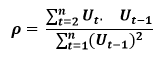
If most of the points fall in the 2nd and 4th quadrant , the autocorrelation will be negative, because the products are negative. By plotting ei against time : The successive values of ei are plotted against time would indicate the possible presence of autocorrelation .If e’s in successive time show a regular time pattern, then there is autocorrelation in the function. The autocorrelation is said to be negative if successive values of ei changes sign frequently. First Order of Autocorrelation (AR-1) When t-1 time period’s error affects the error of time period t (current time period), then it is called first order of autocorrelation. AR-1 coefficient p takes values between +1 and -1 The size of this coefficient p determines the strength of autocorrelation. A positive value of p indicates a positive autocorrelation. A negative value of p indicates a negative autocorrelation In case if p = 0, then this indicates there is no autocorrelation. To explain the error term in any particular period t, we use the following formula:-
Where Vt= a random term which fulfills all the usual assumptions of OLS How to find the value of p?
One can estimate the value of ρ by applying the following formula :-
A time series is a sequence of numerical data in which each item is associated with a particular instant in time. Many sets of data appear as time series: a monthly sequence of the quantity of goods shipped from a factory, a weekly series of the number of road accidents, daily rainfall amounts, hourly observations made on the yield of a chemical process, and so on. Examples of time series abound in such fields as economics, business, engineering, the natural sciences (especially geophysics and meteorology), and the social sciences.
Univariate time series analysis- When we have a single sequence of data observed over time then it is called univariate time series analysis.
Multivariate time series analysis – When we have several sets of data for the same sequence of time periods to observe then it is called multivariate time series analysis.
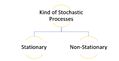
The data used in time series analysis is a random variable (Yt) where t is denoted as time and such a collection of random variables ordered in time is called random or stochastic process.
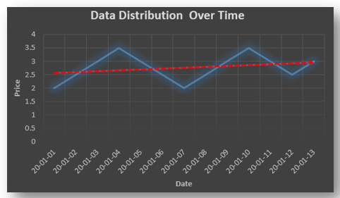
Stationary: A time series is said to be stationary when all the moments of its probability distribution i.e. mean, variance , covariance etc. are invariant over time. It becomes quite easy forecast data in this kind of situation as the hidden patterns are recognizable which make predictions easy.
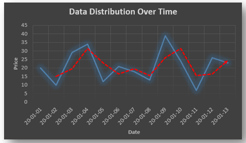
Non-stationary: A non-stationary time series will have a time varying mean or time varying variance or both, which makes it impossible to generalize the time series over other time periods.
Non stationary processes can further be explained with the help of a term called Random walk models. This term or theory usually is used in stock market which assumes that stock prices are independent of each other over time. Now there are two types of random walks: Random walk with drift : When the observation that is to be predicted at a time ‘t’ is equal to last period’s value plus a constant or a drift (α) and the residual term (ε). It can be written as Yt= α + Yt-1 + εt The equation shows that Yt drifts upwards or downwards depending upon α being positive or negative and the mean and the variance also increases over time. Random walk without drift: The random walk without a drift model observes that the values to be predicted at time ‘t’ is equal to last past period’s value plus a random shock. Yt= Yt-1 + εt Consider that the effect in one unit shock then the process started at some time 0 with a value of Y0 When t=1 Y1= Y0 + ε1 When t=2 Y2= Y1+ ε2= Y0 + ε1+ ε2 In general, Yt= Y0+∑ εt In this case as t increases the variance increases indefinitely whereas the mean value of Y is equal to its initial or starting value. Therefore the random walk model without drift is a non-stationary process.
So, with that we come to the end of the discussion on the Time Series. Hopefully it helped you understand time Series, for more information you can also watch the video tutorial attached down this blog. DexLab Analytics offers machine learning courses in delhi. To keep on learning more, follow DexLab Analytics blog.
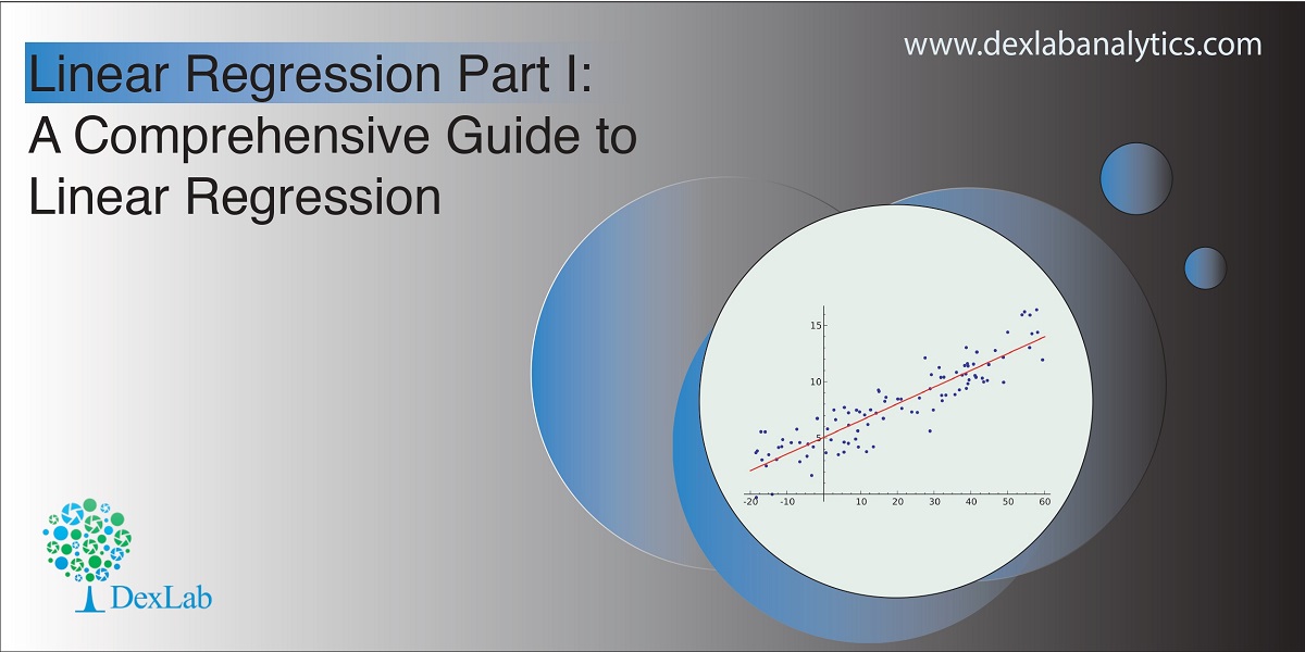
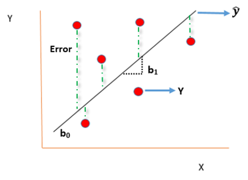
Today’s blog explores another vital statistical concept Linear Regression, let’s begin. Linear regression is normally used in statistics for predictive modeling. It tries to model a relationship between two independent (explanatory variable) and dependent (explained variable) variables X and Y by fitting a linear equation (Y=bo+b1X+Ui) to an observed data.
Assumptions of linear regression
Ui is a random real variable, where Ui is the difference between the observed dependent variable Y and predicted Y variable.
The mean of Ui in any particular period is zero.
The variance of Ui is constant in each period i.e for all values of X, Ui will show the same dispersion around their mean
The variable Ui has a normal distribution i.e the value of Ui (for each Xi) have a bell shaped symmetrical distribution about their zero mean.
The random terms of different observations are independent i.e the covariance of any Ui with any other Uj is equal to zero.
Ui is independent of the explanatory variable X.
Xi are a set of fixed values in the hypothesised process of repeated sampling which underlies the linear regression model.
In case there are more than one explanatory variables then they are not perfectly linearly correlated.
Linear Regression equation can be written as:
Where,
is the dependent variable
X is the independent variable.
b0 is the intercept (where the line crosses the vertical y-axis)
b1 is the slope
Ui is the error term (difference between ) also called residual or white noise.
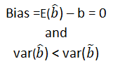
Simple linear regression follows the properties of Ordinary Least Square (OLS) which are as follows:-
Unbiased estimator:- E()=b ie. an estimator is unbiased if its bias is 0; E() – b = 0
Minimum Variance:- An estimate is best when it has the smallest variance as compared to any other estimate obtained from other econometric method.
Efficient estimator:- When it has both the previous properties ie.
Linear estimator
Best, Linear, Unbiased estimator (BLUE)
Minimum mean squared error (MSE) estimator:- It is a combination of the unbiasedness and minimum variance properties. An estimator is a minimum MSE estimator if it has the smallest mean square error.
With that the discussion on Linear Regression wraps up here, hopefully it cleared away any confusion you might have and helped you get a grasp on the concept. We have a video discussion on this same topic, which is attached below this blog, check it out for further reference.
With 2.5 quintillion bytes of data being created everyday companies are scrambling to build models and hire experts to extract information hidden in massive unstructured datasets and the data scientists have become the most sought-after professionals in the world. The job portals are full of job postings looking for data scientists whose resume has the perfect combination of skill and experience. In this world which is being driven by the data revolution, achieving your big data career dreams need a little bit of planning and strategizing. So, here is a step-by-step guide for you.
Grabbing a high paying and skilled data job is not going to be easy, industries will only invest money on individuals with the right skillset. Your job responsibility will involve wading through tons of unstructured data to find pattern and meaning, making forecasts regarding marketing trends, customer behavior and deliver the insight in a presentable format to the company on the basis of which they are going to be strategizing.
So, before you even begin make sure that you have the tenacity and enthusiasm required for the job. You would need to undergo Data science using python training, in order to gain the necessary skills and knowledge and since this is an evolving field you should be ready to constantly upskill yourself and stay updated about the latest developments in the field.
Are you ready? If it’s a resounding yes, then, without wasting any more time let’s get straight to the point and explore the steps that will lead you to become a data scientist.
Step 1: Complete education
Before you pursue data science, you must complete your bachelors degree, if you are coming from computer science, applied mathematics, or, economics that could give you a head start. However, you need to undergo Data Science training, post that to acquire the required skillset.
Step 2: Gain knowledge of Mathematics and statistics
You do not need to have a PHD in either, but, since both are at the core of the data science you must have a good grasp on applied mathematics and statistics. Your task would require you to have knowledge regarding linear algebra, probability & statistics. So, your first step would be to update yourself and be familiar with the concepts if you happen to hail from a non-science background so that you can sail through the rest of the journey.
Step 3: Get ready to do programming
Just like mathematics and statistics, having a grip on a programming language preferably Python, is essential. Now, why do you need to learn coding? Well, coding is important as you have to work with large datasets comprising mostly unstructured data and coding will help you to clean, organize, read data and also process it. Now the stress is on Python because it is one of the widely used languages in the data science community and is comparatively easier to pick up.
Step 4: Learn Machine Learning
Machine learning plays a crucial role in data science as it helps finding patterns in data and making predictions. Mastering machine learning techniques would enable you develop algorithms for the models and create an automated system that enables you to make predictions in real-time. Consider undergoing a Machine Learning training gurgaon.
Step 5: Learn Data Munging, Visualization, and Reporting
It has been mentioned before that you would mostly be handling unstructured data, which means in order to process that data you must transform that data into a format that is easy to work with. Data munging helps you achieve that. Data visualization is again a must-have skill for a data scientist as it allows you to visually present your data findings that is easy to understand through graphs, charts, while data reporting lets you prepare and present reports for businesses.
Step 6: Be certified
Now that the field has advanced so much, there is a requirement for professionals who have undergone Data Science course. Doing a certification course would upskill you and arm you with industry knowledge. Reputed institutes like Dexlab Analytics offer cutting edge courses such as Python for data science training. If you just follow this step it would take care of the rest of the worries, the best part of getting your training is that here you will be taught everything from scratch so, no need to fret if you do not know programming language. Your learning would be aided by hands-on training.
Step 7: Practice your skills
You need to test the skills you have acquired and to hone the skills you must explore Kaggle, which lets your access resources you need and this platform also allows you to take part in competitions that further helps you sharpen your abilities. You should also keep on practicing by doing projects in order to put the theories into action.
Step 8: Work on your soft skills
In order to be a professional data scientist you must acquire soft skills as well. So along with working on your communication skills, you must also need to develop problem solving skills while learning how business organizations function to understand what would be required of you when you assume the role of a data scientist.
Step 9: Get an internship
Now that you have the skill and certification you need experience to get hired, build a resume stressing on the skills you have acquired and search the job portals to land an internship. It would not only enhance your resume, but, it also gives you exposures to real projects, the more projects you handle the better and you would also learn from the experts there.
Step 10: Apply for a job
Once you have gathered enough experience start applying for full-time positions as now you have both skill and experience. But, do not stop learning once you land a job, because this field is growing many changes will happen so you have to mold yourself accordingly. Be a part of the community, network with people, keep on exploring GitHub and find out what other skills you require.
So, those were the steps you need to follow to build a rewarding career in data science. The job opportunities are plenty and to grab the right job you must do big data training in gurgaon. These courses are aimed to prepare individuals for the industry, so get ready for an exciting career!