Credit Risk in Indian Banking: What RBI’s Data Actually Shows
Every risk professional in Indian banking eventually asks the same question: is credit risk actually improving, or does it just look that way in aggregate numbers? Based on the Reserve Bank of India’s own published data, the answer is both. System-wide asset quality has genuinely strengthened over the past five years. But the composition of that risk is shifting in a direction that deserves closer attention.
This piece works through RBI’s Financial Stability Reports (FSR), sectoral credit data, and the newly finalized Expected Credit Loss (ECL) framework. Together they show what’s really happening with credit risk in Indian banking between 2020 and 2025. It does not rely on a proprietary survey or projected estimates dressed up as findings. In fact, every figure below is sourced directly to a named RBI report. That distinction matters: in a domain where regulators, auditors, and rating agencies check your numbers, credibility is the entire product.
Three questions structure the analysis. How has aggregate asset quality moved since the 2020 pandemic shock? Where is risk concentrating today, even as headline numbers improve? And what does the incoming ECL regime signal about how Indian banks will need to manage credit risk going forward?
Methodology and Data Sources
This analysis draws on primary RBI publications, cross-checked across multiple reporting periods for consistency.
RBI Financial Stability Reports (FSR): Published twice yearly. They consolidate Gross NPA (GNPA) and Net NPA (NNPA) ratios of Scheduled Commercial Banks (SCBs), capital adequacy (CRAR), bank-group-wise asset quality, and stress test results. Specifically, this piece uses FSR editions from January 2021 through December 2025.
RBI Sectoral Deployment of Bank Credit data: Monthly data on credit growth to industry, services, agriculture, and personal loans. It’s sourced from 41 banks representing roughly 95% of non-food credit.
RBI’s ECL framework releases: The draft ECL directions (October 2025) and final directions (April 2026). These describe the shift from incurred-loss to forward-looking PD/LGD/EAD-based provisioning, effective April 1, 2027.
One scope note: RBI does not publish a standardized “default rate by loan product” table. Where this article cites loan-category or bank-group figures, they are GNPA ratios: the share of gross advances classified as non-performing. It’s the metric RBI itself uses, and the one directly comparable across periods.
Finding 1: Asset Quality Has Improved for Five Consecutive Years
SCB GNPA: from 8% to 2.1% in five years
Period
GNPA Ratio
NNPA Ratio
Source
March 2020
8.4%
—
RBI FSR, Jan 2021
September 2020
7.5%
—
RBI FSR, Jan 2021
March 2024
2.8%
0.6%
RBI FSR, Jun 2024
March 2025
2.3%
0.5%
RBI FSR, Jun 2025
September 2025
2.1%–2.2%
—
RBI FSR, Dec 2025
March 2027 (projected, baseline)
1.9%
—
RBI FSR, Dec 2025
RBI’s January 2021 report recorded a September 2020 GNPA ratio of 7.5%, down from 8.4% in March 2020. That was a system still absorbing the pandemic shock. GNPA had fallen to 2.8% by June 2024, then to 2.3% by March 2025. It touched a multi-decade low of 2.1% by September 2025, and RBI projects further improvement to 1.9% by March 2027 under its baseline scenario.
In practice, this reflects five years of balance sheet cleanup: post-IBC resolution of legacy corporate stress, tighter underwriting after the 2018–2020 NBFC stress episode, and stronger capital buffers overall. Meanwhile, system-wide CRAR remains comfortably above regulatory minimums, with public sector banks at 16% and private banks at 18.1% as of September 2025.
In short, aggregate GNPA is a lagging confirmation of underwriting discipline, not a leading indicator. A PD model trained mainly on 2020–2022 stressed data will overstate current default risk. One trained only on 2023–2025 benign data risks understating tail risk in the next downturn.
Explore our Credit Risk Modeling Certification Training for a structured approach to PD estimation across credit cycles.
Finding 2: Improvement Isn’t Even Across Bank Groups
PSBs are catching up fast
For instance, PSB GNPA fell sharply from 3.7% in March 2024 to 2.8% in March 2025. Meanwhile, private bank GNPA held roughly stable at 2.8% over the same period, and foreign banks improved from 1.2% to 0.9%.
Even so, this convergence matters. For most of the post-2015 asset-quality-review era, PSB asset quality lagged private banks significantly, largely on corporate exposures. That gap has now nearly closed at the aggregate level. However, remaining risk differs by bank group, which leads to the more consequential finding below.
Finding 3: Unsecured Retail Is Where New Risk Concentrates
The retail risk hiding inside a good headline number
This is the most important finding for practitioners, because it sits underneath the reassuring headline number. According to RBI’s December 2025 FSR, roughly 53.1% of retail loan slippages now originate from unsecured products like personal loans and credit cards. At private banks, unsecured loans account for nearly 76% of fresh slippages. GNPA on unsecured retail loans stood at 1.8%, versus 1.1% for overall retail advances.
In other words, the 2.1% aggregate GNPA figure blends a very clean secured/corporate book with a smaller, faster-deteriorating unsecured retail book. RBI flagged this as a fintech-adjacent risk, tied to fast credit growth in small-ticket personal loans to borrowers under 35 through digital lending channels.
This pattern, in fact, tracks with operational experience. Unsecured lending has weaker recovery mechanics (no collateral to liquidate, higher LGD), shorter behavioral history on new-to-credit borrowers, and faster origination cycles that compress underwriting review. Moreover, it is the segment where forward-looking provisioning matters most, since unsecured risk builds up quietly between formal NPA recognition points.
As a result, portfolio-level GNPA alone is no longer sufficient. Overall, segment-level GNPA and vintage curves for unsecured retail belong alongside the aggregate number in any board-level risk dashboard.
Finding 4: ECL Will Formalize This Shift
Why the 2027 ECL shift matters here
RBI has issued directions introducing forward-looking ECL provisioning, replacing the incurred-loss model. It takes effect April 1, 2027, for scheduled commercial banks excluding RRBs, Small Finance Banks, and payments banks. ECL provisioning must be based on a bank’s own historical PD and LGD data spanning at least five years, subject to RBI-specified floors. Accounts 30–90 days past due move into Stage 2, a materially earlier trigger than the current framework.
Overall, the shift aligns India’s prudential norms with global IFRS 9 standards. In addition, it requires closer integration between finance and risk functions, as forward-looking macroeconomic scenarios become a formal input to provisioning.
Indeed, this is a direct regulatory response to Finding 3. An incurred-loss model recognizes impairment only after default has effectively occurred. ECL requires estimating expected loss, via PD, LGD, and EAD, well before that point, catching unsecured deterioration earlier in the cycle.
Even so, for banks building this capability, it isn’t a compliance task to fully outsource. RBI has explicitly made a bank’s board and senior management responsible for the adequacy of the ECL framework. Consequently, internal teams need working fluency in PD/LGD/EAD construction, not just the ability to read vendor output. However, it’s worth noting that the standard formula, Expected Loss = PD × LGD × EAD, assumes independence between the three components. In practice they’re correlated: LGD tends to rise in the same downturns that push PD higher. That’s why RBI’s stress tests apply adverse scenarios jointly rather than multiplying baseline figures in isolation.
What This Means for Banks and Risk Teams
First, aggregate GNPA improvement is real but incomplete. Segment-level monitoring, especially for unsecured retail, deserves as much attention as the headline ratio.
PD/LGD model recency matters. RBI’s own five-year minimum spans both a stressed period (2020–2021) and a benign one (2023–2025). Models need to represent both.
Collateral still matters, but isn’t the whole story. Unsecured products drive a disproportionate share of new slippages. In turn, this argues for tighter underwriting in that segment, not a wholesale retreat from unsecured lending.
Finally, the 2027 ECL deadline is closer than it looks. In practice, building five years of clean PD/LGD data and validation capability is a multi-year undertaking. Banks starting in 2026 are already behind institutions that began in 2024–2025.
Recovery rate discipline matters for LGD. LGD = 1 − Recovery Rate only holds up when ‘recovery rate’ is the economic, discounted, net-of-cost rate, not the nominal amount eventually collected.
Explore our Credit Risk Modeling Certification Training to build PD, LGD, and EAD modeling skills ahead of the 2027 ECL transition, or see Understanding Credit Risk: Definition and Types for foundational concepts referenced throughout.
FAQ
What is the current GNPA ratio of Indian banks?
As of September 2025, SCB GNPA stood at 2.1%, a multi-decade low, per RBI’s December 2025 Financial Stability Report.
Is unsecured lending riskier than secured lending right now?
Yes, and the gap is widening. Unsecured retail GNPA was 1.8% versus 1.1% for overall retail advances, and unsecured products drove over half of all retail slippages.
When does RBI’s ECL framework take effect?
RBI’s ECL Directions were issued 27 April 2026 and take effect April 1, 2027. They apply to commercial banks, excluding small finance banks, payments banks, and local area banks.
Does EL = PD × LGD × EAD fully capture expected loss?
It’s the standard starting formula, but it assumes PD, LGD, and EAD move independently. In stress, they’re correlated — which is why RBI applies adverse scenarios jointly rather than multiplying baseline values.
Conclusion
The data supports a measured conclusion, not a triumphant one. Indeed, Indian banking’s asset quality genuinely improved for five straight years, and RBI’s own numbers back that up without embellishment. However, the same data shows risk isn’t disappearing. Instead, it’s relocating toward unsecured retail lending, addressed through a regulatory shift that will demand more rigorous PD, LGD, and EAD modeling capability than most institutions currently have in-house. For risk analysts, credit officers, and model validators, that combination is telling: improving headline numbers alongside a harder compliance mandate. It’s exactly why 2025–2027 is a build-capability window, not a wait-and-see one.
This analysis is based on RBI’s Financial Stability Reports, Sectoral Deployment of Bank Credit data, and RBI’s ECL Directions (2025–2026). Figures are reported as published at the cited dates; readers should consult original RBI releases for the most current data.
Ready to Build These Skills Hands-On?
Understanding the theory behind PD, LGD, and EAD is the first step. Building bankable, interview-ready models — in Python or SAS, on real credit datasets, aligned to Basel and IFRS 9 — is what actually moves a career forward.
Explore Dexlab Analytics’ Credit Risk Modeling certification program to build PD, LGD, and EAD models from scratch, work through IFRS 9 ECL frameworks, and learn model validation techniques used by practicing risk teams.
In March 2021, a little-known family office called Archegos Capital Management defaulted on margin calls from its banks. Within days, Credit Suisse lost $5.5 billion. Nomura lost close to $2.5 billion. Morgan Stanley and UBS lost roughly $1 billion and $774 million. Combined, global banks lost more than $10 billion — not because of a market crash, but because of one counterparty’s concentrated, hidden leverage.
That’s credit risk in its purest form. It’s the possibility that someone you’ve extended money or exposure to won’t pay it back, and the cascading damage that follows when large exposures go bad at once.
Most people equate credit risk with loan defaults. That’s only part of the picture. Credit risk shows up in derivatives, trade settlements, corporate bonds, and interbank lending. It appears anywhere one party depends on another to deliver.
This guide breaks down what credit risk actually means. It covers the distinct types every risk professional needs to recognize, and how banks measure and manage it in practice, in India and globally.
What is Credit Risk?
Credit risk is the possibility that a borrower or counterparty fails to meet a financial obligation, causing a loss to the lender. That’s the formal definition. In plain terms: it’s the risk that you lend money, extend credit, or enter a contract with someone, and they don’t hold up their end. The Reserve Bank of India’s Guidance Note on Credit Risk Management frames it more precisely. Credit risk can be an individual transaction risk — the chance that one specific loan goes bad. Or it can be a portfolio risk, which looks at how credit losses behave in aggregate across a bank’s book. A single bad loan is a manageable, expected cost of doing business. Thousands of correlated bad loans, going bad at once because they share a common vulnerability, is a solvency event.
Credit risk isn’t limited to banks lending to individuals or businesses. It appears in:
Loans and advances — the most familiar form, where a borrower fails to repay principal or interest
Bonds and fixed-income securities — where an issuer defaults on coupon payments or principal at maturity
Derivatives contracts — where a counterparty can’t meet its obligations under a swap, option, or forward
Trade finance and settlement — where one party in a transaction fails to deliver cash or securities as agreed
Guarantees and letters of credit — where a bank stands behind another party’s obligation and gets called on to pay
Under the Basel framework, credit risk-weighted assets typically make up the largest share of the capital a bank must hold. That’s larger than market risk or operational risk combined, for most commercial banks. This is why understanding credit risk isn’t a niche specialty. It’s the foundation most of banking risk management sits on.
Types of Credit Risk
Credit risk isn’t one uniform threat. RBI’s own framework splits transaction-level credit risk into default risk and rating migration risk. It splits portfolio-level risk into intrinsic risk and concentration risk. Layered on top of that, banking practice recognizes several distinct sub-types worth understanding individually. Three matter most for anyone building a working knowledge of the field: counterparty risk, concentration risk, and settlement risk.
The distinction isn’t academic. Each type demands a different measurement approach, a different mitigation strategy, and often a different team within a bank’s risk function. A credit officer underwriting a retail loan thinks primarily about default risk on that single borrower. A treasury desk trading derivatives thinks primarily about counterparty risk and daily mark-to-market exposure. A chief risk officer reviewing the whole institution thinks about concentration across the entire book. Does the bank have too much riding on one sector, one region, or one large group of related borrowers? Confusing these categories, or managing them with a single generic framework, is exactly how risks that look small individually compound into something systemic.
Counterparty Risk
Counterparty risk is the risk that the other party in a financial contract fails to fulfill their side of the deal. This isn’t a traditional borrower — it’s a trading or derivatives counterparty. It’s especially relevant in derivatives, securities lending, and prime brokerage relationships. There, exposure isn’t a fixed loan amount. It’s a fluctuating mark-to-market value.
The Archegos collapse is the clearest recent illustration. Archegos used total return swaps to build enormous, concentrated positions in a small number of stocks. It never owned the shares directly, and never disclosed the size of its bets. Its prime brokers — Credit Suisse, Nomura, Morgan Stanley, Goldman Sachs, and UBS — each saw only their own slice of Archegos’s exposure. None had visibility into the full picture. When the fund’s portfolio value fell roughly 30% in four days in March 2021, it couldn’t meet margin calls. Its brokers had to liquidate billions of dollars in positions simultaneously. Those unable to exit fast enough absorbed massive losses.
Analysts who studied the collapse point to a specific, technical failure mode: wrong-way risk. This occurs when a bank’s exposure to a counterparty grows precisely as that counterparty’s ability to pay deteriorates. Archegos’s swap exposure ballooned in tandem with its portfolio’s decline. The worse things got, the more the banks were owed, and the less able Archegos was to cover it. The European Central Bank later reviewed 23 major banks’ derivatives exposures. It found “material shortcomings” in how counterparty credit risk was governed across the industry.
Concentration Risk
Concentration risk arises when a bank’s credit exposure clusters too heavily around a single borrower, sector, geography, or risk factor. Diversification is supposed to protect a lender. If one borrower fails, the loss should be a small fraction of the total book. Concentration undermines that protection entirely.
Archegos illustrates this too, in a second way. The fund’s own portfolio was concentrated in a handful of technology and media stocks. When those specific names fell, there was no offsetting position to cushion the blow. The losses hit every position at once. Banks face the mirror image of this problem in lending. Heavy exposure to one industry, real estate for instance, or one large corporate group, means a single sector downturn can impair a disproportionate share of the loan book. RBI’s prudential framework directly addresses this. It sets single-borrower and group-borrower exposure limits specifically to prevent Indian banks from building the kind of concentrated exposure that made Archegos so dangerous to its lenders.
Settlement Risk
Settlement risk is sometimes called Herstatt risk, after the 1974 collapse of Bankhaus Herstatt. It’s the risk that one party in a transaction delivers its side — cash or securities — while the counterparty fails to deliver theirs. This typically happens because of timing gaps, or the counterparty’s failure between trade execution and final settlement. Herstatt was shut down by German regulators mid-day. By then it had already received Deutsche Mark payments from counterparties, but it hadn’t yet sent back the US dollars it owed in return. Banks on the other side of those foreign exchange trades lost their payments outright.
That single event reshaped global payments infrastructure. It led directly to the creation of CLS Bank, a settlement system designed specifically to eliminate this timing gap in foreign exchange transactions. CLS does this by settling both legs of a trade simultaneously. Settlement risk remains a live concern anywhere payment and delivery aren’t simultaneous. It’s a reminder that credit risk isn’t only about long-term loans — it can materialize in a transaction that’s supposed to finish within hours.
Default Risk Explained
Default risk sits at the center of every credit risk framework. It’s the risk that a borrower simply stops paying. Understanding what causes defaults, and how professionals frame the probability of one occurring, is foundational to everything else in credit risk modeling.
It’s also the oldest form of credit risk banks have grappled with. Long before derivatives, prime brokerage, or cross-border settlement systems existed, lenders were already trying to predict which borrowers would repay and which wouldn’t. Every other risk type covered in this guide is, in some sense, a more specialized variant of the same underlying question: will the party on the other side of this transaction deliver what they owe? Default risk asks that question in its most direct form, applied to a straightforward loan or credit exposure.
What Causes Defaults
Defaults rarely happen for one isolated reason. They typically result from a mix of factors:
Cash flow deterioration. A borrower’s income or business revenue falls below what’s needed to service debt. For individuals, this might mean job loss. For corporates, it might mean a demand shock or margin compression.
Over-leverage. A borrower takes on more debt than their income can realistically support, leaving no buffer when conditions turn even mildly unfavorable.
Macroeconomic shocks. Recessions, interest rate spikes, or sector-wide downturns push otherwise healthy borrowers into distress simultaneously — the mechanism behind concentration risk turning into realized losses.
Governance and fraud. Misrepresented financials, diverted funds, or outright fraud can turn an apparently strong borrower into a default risk overnight. Archegos itself is a governance case as much as a market one — Bill Hwang was later convicted on fraud and racketeering charges tied to how the fund misled its own counterparties about position size and concentration.
Willful default. Occasionally, a borrower who can pay simply chooses not to, usually when the cost of default (reputational or legal) is judged lower than the cost of repayment.
The Probability Framework
Rather than treating default as a binary surprise, credit risk professionals model it as a probability. A Probability of Default (PD) is expressed as a percentage likelihood that a borrower defaults within a defined time horizon, typically 12 months for regulatory purposes. A PD of 2% doesn’t mean a specific borrower is “slightly risky.” It means that, across a large pool of similar borrowers, roughly 2 in 100 are expected to default within that window.
This probabilistic framing matters. It converts an unpredictable individual event into something a bank can price, provision for, and manage at portfolio scale. Building a reliable PD estimate is a discipline in its own right — deciding which borrower characteristics matter, which statistical technique to use, and how to validate the result. We cover the full methodology, including logistic regression and survival analysis, in our detailed guide to PD estimation.
What matters at this stage is the underlying logic: default isn’t modeled as a yes/no outcome for an individual borrower. It’s modeled as a rate across a population, calibrated against historical data and adjusted for current conditions.
Credit Risk in International Banking
Credit risk doesn’t stop at national borders, and neither does its regulation. Two frameworks matter most for anyone working in or around Indian banking. One is the International Accounting Standards Board’s approach to credit loss recognition. The other is RBI’s domestic prudential framework.
Why does a domestic Indian bank need to care about an international accounting standard? Because capital markets are global, even when a bank’s loan book isn’t. Foreign investors, rating agencies, and cross-border lenders all benchmark a bank’s provisioning and capital adequacy against international norms, whether or not that bank operates outside India. A framework that looks conservative by domestic standards can still look under-provisioned by global standards. That gap shows up directly in borrowing costs, credit ratings, and investor confidence.
The IASB and IFRS 9
The International Accounting Standards Board (IASB) issued IFRS 9 specifically to fix a weakness exposed by the 2008 financial crisis. The old “incurred loss” model only recognized credit losses after a default had already happened — by which point it was too late for provisions to cushion the blow. IFRS 9 replaced that with an Expected Credit Loss (ECL) model. It requires banks to recognize losses based on forward-looking estimates, before default occurs. IFRS 9 has been adopted across more than 140 jurisdictions worldwide, making it one of the most widely applied accounting standards in global banking.
RBI’s Framework and India’s ECL Transition
India has historically run on a different system: the Income Recognition and Asset Classification (IRAC) norms. These classify loans as standard, sub-standard, doubtful, or loss, based on how many days they’re overdue, and provision accordingly. That’s closer to the old “incurred loss” approach IFRS 9 was designed to replace.
That’s now changing. RBI has confirmed that an ECL-based provisioning framework, with prudential floors, will apply to all Scheduled Commercial Banks from April 1, 2027. Under the new norms, banks will classify financial assets into Stage 1, Stage 2, or Stage 3. That classification depends on assessed credit losses at initial recognition, and at each subsequent reporting date — directly mirroring the IFRS 9 structure used globally.
RBI has also been actively updating its credit risk rules to align with Basel Committee on Banking Supervision (BCBS) standards. In 2026, it revised its counterparty credit risk framework specifically to bring India’s derivatives exposure measurement closer to global norms. That’s a change regulators internationally have prioritized in the years following the Archegos collapse. India’s Capital-to-Risk-Weighted-Assets Ratio (CRAR) requirement of 9% for scheduled commercial banks also exceeds the 8% global Basel III minimum. That reflects RBI’s consistently more conservative capital stance relative to international baselines.
Measuring Credit Risk
Defining and categorizing credit risk only gets a risk team so far. Managing it requires quantifying it — turning a qualitative concern into numbers that inform pricing, provisioning, and capital decisions. Four metrics form the core toolkit.
Probability of Default (PD)
As covered above, PD is the percentage likelihood that a borrower defaults within a set time horizon. It’s typically estimated through logistic regression or survival analysis, using historical repayment data, bureau scores, and financial ratios as inputs. PD is the starting point for nearly every downstream credit risk calculation.
Loss Given Default (LGD)
Default doesn’t automatically mean total loss. LGD measures the proportion of exposure a lender expects to actually lose after accounting for recoveries — collateral liquidation, guarantees, or restructuring. Getting LGD right requires more care than it first appears. It has to reflect the economic recovery rate, discounted for the time value of money and net of recovery costs — not just the raw cash eventually collected. A recovery that takes three years to materialize is worth meaningfully less than the same amount recovered immediately.
Credit Ratings
Credit ratings translate a borrower’s creditworthiness into a standardized letter grade, from investment-grade (AAA down to BBB-) to speculative or junk grades below that. In India, these come from agencies like CRISIL, ICRA, and CARE; internationally, from S&P, Moody’s, and Fitch. Ratings aren’t a substitute for internal PD modeling. But they serve two practical purposes. They give banks an independent, externally validated view of risk. And they directly feed into regulatory risk-weighting under the Basel Standardised Approach, where a lower rating translates into a higher capital charge against that exposure.
Expected Loss and Exposure at Default (EAD)
Exposure at Default (EAD) measures how much a lender is actually on the hook for at the moment a default happens. For revolving credit like credit cards, this can run higher than the current outstanding balance, since distressed borrowers often draw down more of their available limit before defaulting. Combining EAD with PD and LGD produces Expected Loss (EL) — the amount a bank should provision for a given exposure on average. It’s worth noting this combined figure is a standard industry simplification. It assumes PD, LGD, and EAD move independently, which understates risk in downturns, when all three tend to move against the lender simultaneously. Regulators address this specific gap by requiring “downturn” LGD and EAD estimates, rather than accepting benign-cycle averages alone.
Used together, these four metrics let a bank move from “this borrower feels risky” to a specific number. That number can be priced into a loan, provisioned for on the balance sheet, and reported to regulators with a defensible methodology behind it.
Conclusion
Credit risk is broader and more structured than “will this loan get repaid.” It spans counterparty exposure in derivatives, concentration across a portfolio, settlement timing in payments, and default at the level of an individual borrower. Each has distinct causes, distinct historical failures, and distinct measurement approaches. Understanding what is credit risk at this level of detail is the foundation every subsequent risk modeling technique builds on, from PD estimation through to full expected-loss calculation.
The Archegos collapse, the 2027 shift to ECL-based provisioning in India, and RBI’s ongoing alignment with Basel counterparty risk standards all point to the same conclusion. Credit risk management is not static. It evolves in direct response to the failures that expose its gaps.
Explore our Credit Risk Modeling Certification Training to master Risk Analytics. Build the PD, LGD, and EAD models covered here from scratch. Work through India’s transition to ECL provisioning, and learn the model validation techniques practicing risk teams use every day.
A practical framework for PD, LGD, EAD and expected loss modeling in banking
Introduction
Between March 2018 and March 2021, gross non-performing assets at India’s public sector banks fell from a peak of 14.58% to 9.11% of advances. By September 2025, the system-wide gross NPA ratio for all scheduled commercial banks had dropped further, to a multi-decade low of 2.15%. That turnaround wasn’t accidental. Tighter underwriting, RBI’s Asset Quality Review, the Insolvency and Bankruptcy Code, and — underlying all of it — better credit risk models drove it.
The lesson for anyone building a career in banking analytics is straightforward. Credit risk is the single largest risk category banks carry on their balance sheets. How well a bank measures it directly determines capital adequacy, profitability, and long-term survival. A bank that underestimates default risk lends into losses it didn’t provision for. A bank that overestimates it prices good borrowers out of the market and loses share to competitors.
This guide walks through the complete framework professionals use to model credit risk. It covers the regulatory logic that makes credit risk modeling non-negotiable. It covers the three parameters that quantify it — PD, LGD, EAD. And it covers the statistical and machine learning techniques used to estimate each one. Maybe you’re a risk analyst preparing for an FRM exam. Maybe you’re a data scientist moving into banking analytics. Maybe you’re evaluating a credit risk modeling certification. Either way, this article builds the structured foundation technical interviews and real project work both expect.
By the end, you’ll understand the formulas. You’ll understand why each one exists, how professionals estimate it in practice, and where Indian banks apply it today.
What is Credit Risk and Why It Matters
Credit risk is the possibility that a borrower fails to meet a contractual debt obligation. The borrower could be an individual, a company, or a counterparty. Either way, it results in a financial loss for the lender. It is the risk that repayment doesn’t happen as agreed: a missed EMI, a defaulted corporate bond, a counterparty that can’t settle a derivative contract.
For a bank, credit risk isn’t one risk among many — it’s usually the dominant one. Loans and advances typically make up the largest share of a bank’s assets. Under the Basel framework, credit risk-weighted assets (RWA) form the biggest component of the capital a bank must hold. When credit risk is mismeasured, everything built on top of that measurement goes wrong too: capital adequacy ratios, loan pricing, provisioning, dividend capacity.
Why Credit Risk Modeling Matters to a Bank’s Survival
Three consequences flow directly from how well a bank models credit risk:
Capital adequacy. Under Basel III, banks must hold capital proportional to the risk-weighted value of their assets. The Capital-to-Risk-Weighted-Assets Ratio (CRAR) for India’s scheduled commercial banks stood at a strong 17.2% as of September 2025 — well above the regulatory minimum. Risk measurement and provisioning discipline improved sharply after 2015, and it shows.
Provisioning under IFRS 9. IFRS 9 replaced the incurred-loss model with an expected credit loss (ECL) model. Banks must now recognize losses before a default happens, based on modeled probabilities. That makes credit risk models a direct input into the profit and loss statement, not just a back-office risk tool.
Pricing and portfolio strategy. A bank that can accurately rank borrowers by risk can price loans correctly, set appropriate limits, and choose which segments to grow or shrink. A bank that can’t ends up either losing good customers to competitors with sharper pricing, or accumulating bad loans that eventually show up as NPAs.
The RBI Regulatory Backdrop
The Reserve Bank of India has steadily tightened the credit risk framework banks operate under. Its 2015 Asset Quality Review forced transparent recognition of stressed assets that restructuring had previously hidden. More recently, in November 2023, the RBI raised risk weights on unsecured consumer credit — from 100% to 125% for banks. NBFC exposures saw a further increase. The goal: curb underpriced risk-taking in retail lending. The RBI has also begun articulating principle-based guidance for AI use in credit decisioning through its evolving regulatory framework. Model governance, not just model accuracy, is now squarely on the regulator’s radar.
This regulatory environment is precisely why credit risk modeling has become a core competency banks and NBFCs actively hire for — not an optional analytics add-on.
Core Components of Credit Risk Modeling
Every credit risk model, regardless of the statistical technique behind it, answers one question: how much money could the bank lose on this exposure, and how likely is that loss?
The industry-standard approach breaks “expected loss” into three independently modeled components:
1. Probability of Default (PD)
PD is the likelihood that a borrower will fail to meet their obligations within a defined time horizon. That’s typically 12 months for regulatory capital purposes, or lifetime PD under IFRS 9 for certain asset stages. PD is expressed as a percentage. A PD of 3% means a 3% chance of default within the horizon, based on the borrower’s characteristics.
2. Loss Given Default (LGD)
Default doesn’t always mean total loss. If a borrower defaults, the bank usually recovers something — through collateral liquidation, guarantees, or restructuring. LGD is the proportion of the exposure the bank expects to actually lose after recoveries. It’s expressed as a percentage of the exposure. An LGD of 40% means that, on average, the bank recovers 60% of what it’s owed after a default.
3. Exposure at Default (EAD)
EAD is the total value the bank carries at the moment of default — not the sanctioned limit, but the amount actually outstanding. For a term loan, this is close to the outstanding balance. Revolving facilities like credit cards or cash credit limits work differently. There, EAD must account for the possibility that the borrower draws down more of the limit before defaulting.
Putting It Together: Expected Loss
These three parameters combine into the foundational credit risk formula:
Expected Loss (EL) = PD × LGD × EAD
Consider a simple example: a bank has an outstanding exposure (EAD) of ₹1 crore to a borrower with a PD of 4% and an LGD of 45%.
Expected Loss = 0.04 × 0.45 × ₹1,00,00,000 = ₹1,80,000
This ₹1.8 lakh isn’t a one-off loss estimate for a single account. It’s the amount the bank should provision for, on average, across a portfolio of similar loans. Multiply this calculation across thousands of accounts, segmented by product, geography, and borrower type. The result is a portfolio-level expected loss figure that feeds directly into provisioning, pricing, and capital planning.
Why This Formula Is a Simplification
EL = PD × LGD × EAD is the standard, industry-wide formula — it’s not wrong. But it rests on an assumption worth naming explicitly: that PD, LGD, and EAD are independent of one another. In reality they aren’t. Recoveries tend to get worse exactly when default rates spike, because both track the same macroeconomic cycle. A recession depresses collateral values and pushes more borrowers into default at the same time. Multiplying three independent point estimates understates loss in exactly the scenarios that matter most. That’s why regulators require downturn LGD and downturn EAD/CCF add-ons rather than accepting benign-cycle averages.
From Single-Period EL to Lifetime ECL
The formula above is also a single-period number, typically 12 months. Under IFRS 9, lifetime ECL for Stage 2 and Stage 3 assets isn’t one multiplication. It’s a discounted sum of marginal expected losses across every remaining period of the loan’s life:
That distinction matters in practice. A 12-month EL figure and a lifetime ECL figure for the same loan can differ substantially. Conflating the two is a common — and consequential — modeling error.
Each of the three components — probability of default, loss given default, and EAD — demands its own data, statistical techniques, and validation standards. Getting the overall expected loss number right depends entirely on getting each of these three right individually. It also depends on staying honest about where the simplifying assumptions break down.
Probability of Default (PD) Estimation
PD estimation is where most credit risk modeling careers begin, because it has the richest data history and the most mature statistical toolkit.
The Data Foundation
PD models draw on historical loan performance data: borrower demographics, financial ratios, repayment history, bureau scores (like CIBIL in India), and macroeconomic variables. The target variable is binary. Did the borrower default within the observation window, typically defined as 90 days past due (DPD), or not?
Method 1: Logistic Regression
Logistic regression remains the industry workhorse for PD modeling, and for good reason. It’s interpretable, regulator-friendly, and produces a probability output directly — exactly what PD requires.
The logistic regression model estimates:
PD = 1 / (1 + e^-(β₀ + β₁X₁ + β₂X₂ + … + βₙXₙ))
X₁ through Xₙ are borrower characteristics: debt-to-income ratio, bureau score, vintage, loan-to-value ratio, and so on. Analysts estimate the β coefficients from historical default data.
Worked example: Suppose a simplified model uses two variables — bureau score and debt-to-income (DTI) ratio — and produces this equation:
PD = 1 / (1 + e^17.165) ≈ 0.00003, or effectively near-zero risk — consistent with a strong bureau score and moderate leverage.
In practice, banks convert these raw PD outputs into a credit scorecard. It’s a points-based system: each variable band — score range, income bracket, tenure — contributes points that sum to a final score. That score maps back to a PD and a risk grade, AAA to D for instance. Most retail lending decision engines run on exactly this system.
Method 2: Survival Analysis
Logistic regression answers “will this borrower default within 12 months?” It doesn’t naturally answer “when.” Survival analysis models the time to default instead, using techniques like the Cox Proportional Hazards model or Kaplan-Meier estimation. It treats default as an “event.” It treats non-defaulted, still-active loans as “censored” observations.
This matters for two practical reasons. First, it lets banks estimate lifetime PD curves, which IFRS 9 requires for Stage 2 and Stage 3 assets. Second, it naturally handles loans that are still performing at the end of the observation period. It doesn’t treat them as “non-defaults” the way a simple logistic model would. That subtlety matters a great deal in mortgage and long-tenure corporate lending portfolios.
Machine Learning Extensions
Random forests, gradient boosting (XGBoost, LightGBM), and neural networks increasingly supplement — not always replace — logistic regression. This works particularly well where alternative data is available: transaction behavior, digital footprint, utility payment history. Industry research on large Indian banks backs this up. ML models can improve default prediction accuracy over ratio-based or bureau-only assessments, particularly for thin-file borrowers without a long credit history. The trade-off is interpretability. Regulators and internal model validation teams expect PD models to be explainable. That’s why techniques like SHAP (SHapley Additive exPlanations) have become standard for justifying ML-based PD outputs to auditors and regulators.
Common Mistakes in PD Modeling
Treating bureau score as a sufficient standalone predictor without controlling for portfolio-specific behavior
Ignoring population stability — a PD model trained on pre-pandemic data can be badly miscalibrated for a post-pandemic portfolio
Failing to account for right-censoring when using a fixed observation window
Overfitting on a small default sample, which is common in low-default portfolios like corporate or sovereign lending
Loss Given Default (LGD) and Recovery
PD tells you whether a loss will happen. LGD tells you how big it will be once it does. Most practitioners consider it the harder of the two to model well. Default events are relatively rare, and recovery processes can take years to conclude.
What Drives LGD
LGD is shaped primarily by three factors:
Collateral coverage and quality. A secured home loan with a well-documented, liquid property as collateral typically carries a far lower LGD than an unsecured personal loan. The reason: the bank has a tangible asset to recover value from.
Seniority of claim. In corporate lending, senior secured lenders recover more than subordinated or unsecured creditors in a resolution or liquidation.
Recovery mechanism and timeline. In India, recovery routes include SARFAESI Act enforcement, Debt Recovery Tribunals, and the Insolvency and Bankruptcy Code (IBC). These matter enormously for LGD estimation. IBC-driven recoveries have averaged around 94% of the fair value of resolved businesses, though considerably less against the original claim amount. System-wide NPA recovery rates for scheduled commercial banks have roughly doubled, from 13.2% in FY18 to 26.2% in FY25, reflecting stronger legal recovery infrastructure.
The Recovery Rate Relationship
LGD and recovery rate are two sides of the same coin:
LGD = 1 − Recovery Rate
That relationship is correct. But it’s easy to misapply, because “recovery rate” is doing a lot of work in that equation. It has to mean the economic recovery rate: the present value of net recoveries, after two adjustments. First, discount every recovered cash flow back to the default date, to account for the time value of money. Second, subtract the direct and indirect costs of recovery — legal fees, collateral liquidation costs, workout team overhead. A workout can take two to three years in India, even under IBC timelines. A rupee recovered in year three is worth meaningfully less than a rupee recovered on day one.
The common mistake: using the nominal recovery rate instead. That’s raw cash eventually recovered, divided by exposure, with no discounting and no cost deduction. It overstates the recovery rate and, by direct consequence, understates LGD. Say a bank nominally recovers 65% of exposure post-default, but that recovery arrives over three years and costs 8% of exposure in legal and liquidation expenses. The economic recovery rate falls well below 65%. The resulting LGD lands correspondingly higher than the naive “35%” the nominal figure would suggest.
Collateral Valuation
For secured lending, LGD modeling starts with realistic collateral valuation — not the value at origination, but the expected value at the time of liquidation, discounted for:
Market depreciation of the asset class (property, equipment, vehicles)
Haircut for forced-sale conditions versus fair market value
Time-to-recovery, since a three-year legal process erodes present value even if the nominal recovery is high
Direct recovery costs (legal fees, auctioneer fees, administrative costs)
Statistical Methods for LGD
Workout LGD (the standard approach): Banks track every actual default in their historical data. They record all cash flows recovered post-default: collateral sale proceeds, settlement payments, guarantee invocations. Then they discount those cash flows back to the default date, using an appropriate discount rate, and net off recovery costs. This produces an empirical, account-level LGD. Analysts then average and segment it by product, collateral type, and vintage.
Regression-based LGD models: Raw workout LGD is bounded between 0 and 1. It can occasionally exceed 1, when recovery costs surpass recoveries. Banks often use techniques suited to bounded outcomes instead. One option is beta regression. Another is a two-stage model: first predict whether any recovery occurs at all, then model the recovery amount conditional on recovery happening.
Downturn LGD: Basel requires banks to estimate LGD under economic downturn conditions, not just average conditions, because collateral values and recovery rates both tend to fall exactly when default rates rise. This is a critical, frequently underestimated requirement. An LGD model calibrated only on benign-cycle data will understate loss severity in a stress scenario.
A Practical Note on LGD in Indian Retail Lending
For Indian home loans, LGD modeling relies heavily on loan-to-value (LTV) ratio at origination and current LTV, adjusted for property price movements. Property is the dominant recovery source here. Unsecured personal loans and credit cards work differently — they carry substantially higher and more volatile LGD, since recovery depends almost entirely on borrower cooperation, collection agency effectiveness, or write-off. That’s part of why the RBI’s 2023 risk-weight increase on unsecured credit targeted loss severity concerns explicitly. <h2id=”exposure-at-default”>Exposure at Default (EAD) Calculation
EAD often gets treated as the “simple” component of the PD × LGD × EAD formula, but any product with a revolving or undrawn component needs its own careful modeling.
Why EAD Isn’t Just the Current Balance
For a fully drawn term loan, EAD is straightforward. It stays close to the outstanding principal balance at any point in time, adjusted for scheduled amortization. Products like credit cards, overdrafts, and cash credit facilities work differently. A borrower can draw down additional funds between the assessment date and the moment of default. A borrower approaching financial distress often draws their credit line closer to the limit right before defaulting. That means EAD tends to run higher than the current outstanding balance, for exactly the accounts where it matters most.
The Credit Conversion Factor (CCF)
To capture this, banks use the Credit Conversion Factor (CCF) — the proportion of the currently undrawn commitment they expect to see drawn down before default.
EAD = Current Outstanding Balance + (CCF × Undrawn Commitment)
Worked example: A borrower has a credit card with a sanctioned limit of ₹5,00,000. The current outstanding balance is ₹2,00,000, leaving an undrawn commitment of ₹3,00,000. Historical data shows that, on average, borrowers who eventually default draw down 60% of their remaining undrawn limit before the default event (CCF = 0.60).
This runs meaningfully higher than the ₹2,00,000 current balance. The expected loss calculation should use the ₹3,80,000 figure, not the current balance.
How CCF Is Estimated
Banks typically estimate CCF empirically, using a cohort approach. They identify accounts that defaulted. They look back at each account’s utilization level 12 months before default. Then they measure how much of the then-undrawn limit got drawn down by the time of default. Averaging this ratio across the portfolio — segmented by product type and current utilization band — produces the CCF estimates that feed EAD models.
CCF runs highest for revolving retail products like credit cards and overdrafts. It runs near-zero for term loans with no undrawn component. Corporate revolving credit facilities and working capital limits also require dedicated CCF modeling. Distressed corporate borrowers frequently draw down committed but unused credit lines as a liquidity buffer before default becomes evident.
EAD Under Basel and IFRS 9
Under the Basel Internal Ratings-Based (IRB) approach, EAD estimation follows the same downturn-conditioning logic as LGD. CCFs should reflect what happens under stressed conditions, since utilization tends to spike precisely when the broader environment deteriorates. Under IFRS 9, EAD projections also need to extend across the lifetime of the facility for Stage 2 and Stage 3 exposures, not just a fixed 12-month window.
Real-World Implementation in Banking
The theory behind PD, LGD, and EAD only matters if it translates into disciplined implementation. India’s banking sector over the past decade offers a clear illustration of what that looks like at scale.
The Turnaround in Numbers
Following the RBI’s 2015 Asset Quality Review, public sector banks’ gross NPA ratio rose sharply, as transparent recognition brought hidden stress to light. It peaked at 14.58% in March 2018. What followed was a sustained, model-driven cleanup. Recapitalization, tighter underwriting standards, and the Insolvency and Bankruptcy Code combined to bring the PSB gross NPA ratio down to 9.11% by March 2021, and further to 2.58% by March 2025. System-wide, across all scheduled commercial banks, the gross NPA ratio reached a multi-decade low of around 1.8%–2.15% through late 2025 and into 2026, per the RBI’s Financial Stability Report.
At the institution level, this shows up clearly in individual bank results. For the quarter ended March 2026, State Bank of India — India’s largest lender — reported a gross NPA ratio of 1.49% and a net NPA ratio of 0.39%. HDFC Bank reported a gross NPA ratio of 1.15% and net NPA ratio of 0.38%. These aren’t accidents of a benign credit cycle alone. They reflect years of investment: early warning systems, scorecard-based underwriting, stressed-asset monitoring infrastructure.
What Changed Operationally
Three implementation shifts are consistently cited across the sector:
Early Warning Systems (EWS). Public sector banks have rolled out automated EWS frameworks with roughly 80 distinct triggers. These pull in third-party data to flag stress in borrowing accounts before they slip into NPA status. This shifts credit risk management from reactive classification to proactive monitoring.
Machine learning-augmented scorecards. Industry research examining major Indian banks — SBI, HDFC, ICICI, Kotak Mahindra — found that machine learning techniques consistently outperform pure ratio-based or bureau-score-only assessments. The winning combination: logistic regression alongside random forests and neural networks, incorporating alternative data like transaction behavior and digital usage patterns. It works especially well for borrowers with thin credit files.
Faster, more granular underwriting. The same research found loan approval times at many Indian banks have compressed, from several days to a matter of minutes for eligible segments. Automated, model-based decisioning drives this, rather than manual file review. That shift only became possible once PD and exposure models earned enough validated trust to run with minimal manual override.
The Governance Layer
None of this works without governance. The RBI’s ongoing regulatory review — including its recently articulated principle-based framework for AI use in banking — signals something important. As banks lean further into ML-driven credit risk models, model validation, explainability, and monitoring will matter as much as raw predictive accuracy. A model that can’t be explained to an auditor or regulator can’t be deployed at scale in a regulated balance sheet, no matter how well it performs statistically.
Interview Questions to Test Your Understanding
Write out the expected loss formula and explain what each component represents.
Why is logistic regression still preferred over more complex ML models for regulatory PD models?
What’s the difference between workout LGD and downturn LGD, and why does Basel require the latter?
Explain why EAD for a credit card is typically higher than the current outstanding balance.
How would you validate a PD model’s performance? (Hint: think Gini coefficient, KS statistic, and calibration testing.)
Summary
Credit risk modeling breaks down a complex question: how much could a bank lose, and how likely is it? It splits that question into three independently estimated, rigorously validated components — Probability of Default, Loss Given Default, and Exposure at Default — combined through EL = PD × LGD × EAD. Analysts typically estimate PD through logistic regression and survival analysis, increasingly supplemented by explainable machine learning. LGD depends on collateral quality, recovery mechanisms, and downturn conditions. EAD requires modeling credit conversion factors for any revolving exposure. Together, these three parameters drive capital adequacy, IFRS 9 provisioning, and loan pricing. India’s banking sector’s asset quality turnaround over the past decade proves the point: disciplined credit risk modeling delivers at scale.
Frequently Asked Questions
Q1. What is the difference between credit risk and credit risk modeling?
Credit risk is the underlying possibility of borrower default. Credit risk modeling is the quantitative discipline of measuring that risk. It uses statistical and machine learning techniques to estimate PD, LGD, and EAD, so a bank can price, provision for, and manage the risk.
Q2. Is credit risk modeling the same as credit scoring?
Credit scoring is a subset of credit risk modeling, focused specifically on PD estimation for underwriting decisions. Full credit risk modeling also covers LGD, EAD, portfolio-level expected loss, stress testing, and regulatory capital calculation.
Q3. Which technique is better for PD modeling: logistic regression or machine learning?
Neither wins universally. Logistic regression remains preferred for regulatory capital models, thanks to its interpretability and regulator familiarity. Machine learning models can improve accuracy, particularly with alternative data. But they require additional explainability tooling — like SHAP — to meet governance and audit requirements.
Q4. What skills do I need to build a career in credit risk modeling?
You need statistics (logistic regression, survival analysis), proficiency in Python or SAS, familiarity with Basel and IFRS 9, and hands-on exposure to real credit datasets. Structured training that pairs regulatory context with practical model-building is generally the fastest path in.
Q5. How is credit risk modeling connected to IFRS 9?
IFRS 9 requires banks to recognize expected credit losses using forward-looking PD, LGD, and EAD estimates, rather than waiting for an actual default. Stage 1 assets use a 12-month figure, close to the standard EL = PD × LGD × EAD calculation. Stage 2 and 3 assets use lifetime ECL instead — a discounted sum of marginal expected losses across the loan’s remaining life, not a single multiplication.
Ready to Build These Skills Hands-On?
Understanding the theory behind PD, LGD, and EAD is the first step. Building bankable, interview-ready models — in Python or SAS, on real credit datasets, aligned to Basel and IFRS 9 — is what actually moves a career forward.
Explore Dexlab Analytics’ Credit Risk Modeling certification program to build PD, LGD, and EAD models from scratch, work through IFRS 9 ECL frameworks, and learn model validation techniques used by practicing risk teams.
Data Smoothing is done to better understand the hidden patterns in the data. In the non- stationary processes, it is very hard to forecast the data as the variance over a period of time changes, therefore data smoothing techniques are used to smooth out the irregular roughness to see a clearer signal.
In this segment we will be discussing two of the most important data smoothing techniques :-
Moving average smoothing
Exponential smoothing
Moving average smoothing
Moving average is a technique where subsets of original data are created and then average of each subset is taken to smooth out the data and find the value in between each subset which better helps to see the trend over a period of time.
Lets take an example to better understand the problem.
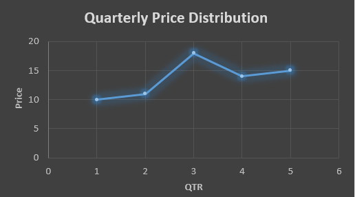
Suppose that we have a data of price observed over a period of time and it is a non-stationary data so that the tend is hard to recognize.
QTR (quarter)
Price
1
10
2
11
3
18
4
14
5
15
6
?
In the above data we don’t know the value of the 6th quarter.
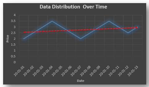
….fig (1)
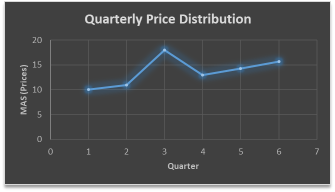
The plot above shows that there is no trend the data is following so to better understand the pattern we calculate the moving average over three quarter at a time so that we get in between values as well as we get the missing value of the 6th quarter.
To find the missing value of 6th quarter we will use previous three quarter’s data i.e.
MAS = = 15.7
QTR (quarter)
Price
1
10
2
11
3
18
4
14
5
15
6
15.7
MAS = = 13
MAS = = 14.33
QTR (quarter)
Price
MAS (Price)
1
10
10
2
11
11
3
18
18
4
14
13
5
15
14.33
6
15.7
15.7
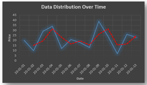
….. fig (2)
In the above graph we can see that after 3rd quarter there is an upward sloping trend in the data.
Exponential Data Smoothing
In this method a larger weight ( ) which lies between 0 & 1 is given to the most recent observations and as the observation grows more distant the weight decreases exponentially.
The weights are decided on the basis how the data is, in case the data has low movement then we will choose the value of closer to 0 and in case the data has a lot more randomness then in that case we would like to choose the value of closer to 1.
EMA= Ft= Ft-1 + (At-1 – Ft-1)
Now lets see a practical example.
For this example we will be taking = 0.5
Taking the same data……
QTR (quarter)
Price
(At)
EMS Price(Ft)
1
10
10
2
11
?
3
18
?
4
14
?
5
15
?
6
?
?
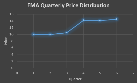
To find the value of yellow cell we need to find out the value of all the blue cells and since we do not have the initial value of F1 we will use the value of A1. Now lets do the calculation:-
F2=10+0.5(10 – 10) = 10
F3=10+0.5(11 – 10) = 10.5
F4=10.5+0.5(18 – 10.5) = 14.25
F5=14.25+0.5(14 – 14.25) = 14.13
F6=14.13+0.5(15 – 14.13)= 14.56
QTR (quarter)
Price
(At)
EMS Price(Ft)
1
10
10
2
11
10
3
18
10.5
4
14
14.25
5
15
14.13
6
14.56
14.56
In the above graph we see that there is a trend now where the data is moving in the upward direction.
So, with that we come to the end of the discussion on the Data smoothing method. Hopefully it helped you understand the topic, for more information you can also watch the video tutorial attached down this blog. The blog is designed and prepared by Niharika Rai, Analytics Consultant, DexLab AnalyticsDexLab Analytics offers machine learning courses in Gurgaon. To keep on learning more, follow DexLab Analytics blog.
A time series is a sequence of numerical data in which each item is associated with a particular instant in time. Many sets of data appear as time series: a monthly sequence of the quantity of goods shipped from a factory, a weekly series of the number of road accidents, daily rainfall amounts, hourly observations made on the yield of a chemical process, and so on. Examples of time series abound in such fields as economics, business, engineering, the natural sciences (especially geophysics and meteorology), and the social sciences.
Univariate time series analysis- When we have a single sequence of data observed over time then it is called univariate time series analysis.
Multivariate time series analysis – When we have several sets of data for the same sequence of time periods to observe then it is called multivariate time series analysis.
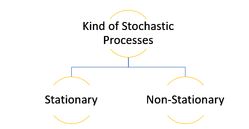
The data used in time series analysis is a random variable (Yt) where t is denoted as time and such a collection of random variables ordered in time is called random or stochastic process.
Stationary: A time series is said to be stationary when all the moments of its probability distribution i.e. mean, variance , covariance etc. are invariant over time. It becomes quite easy forecast data in this kind of situation as the hidden patterns are recognizable which make predictions easy.
Non-stationary: A non-stationary time series will have a time varying mean or time varying variance or both, which makes it impossible to generalize the time series over other time periods.
Non stationary processes can further be explained with the help of a term called Random walk models. This term or theory usually is used in stock market which assumes that stock prices are independent of each other over time. Now there are two types of random walks: Random walk with drift : When the observation that is to be predicted at a time ‘t’ is equal to last period’s value plus a constant or a drift (α) and the residual term (ε). It can be written as Yt= α + Yt-1 + εt The equation shows that Yt drifts upwards or downwards depending upon α being positive or negative and the mean and the variance also increases over time. Random walk without drift: The random walk without a drift model observes that the values to be predicted at time ‘t’ is equal to last past period’s value plus a random shock. Yt= Yt-1 + εt Consider that the effect in one unit shock then the process started at some time 0 with a value of Y0 When t=1 Y1= Y0 + ε1 When t=2 Y2= Y1+ ε2= Y0 + ε1+ ε2 In general, Yt= Y0+∑ εt In this case as t increases the variance increases indefinitely whereas the mean value of Y is equal to its initial or starting value. Therefore the random walk model without drift is a non-stationary process.
So, with that we come to the end of the discussion on the Time Series. Hopefully it helped you understand time Series, for more information you can also watch the video tutorial attached down this blog. DexLab Analytics offers machine learning courses in delhi. To keep on learning more, follow DexLab Analytics blog.
With 2.5 quintillion bytes of data being created everyday companies are scrambling to build models and hire experts to extract information hidden in massive unstructured datasets and the data scientists have become the most sought-after professionals in the world. The job portals are full of job postings looking for data scientists whose resume has the perfect combination of skill and experience. In this world which is being driven by the data revolution, achieving your big data career dreams need a little bit of planning and strategizing. So, here is a step-by-step guide for you.
Grabbing a high paying and skilled data job is not going to be easy, industries will only invest money on individuals with the right skillset. Your job responsibility will involve wading through tons of unstructured data to find pattern and meaning, making forecasts regarding marketing trends, customer behavior and deliver the insight in a presentable format to the company on the basis of which they are going to be strategizing.
So, before you even begin make sure that you have the tenacity and enthusiasm required for the job. You would need to undergo Data science using python training, in order to gain the necessary skills and knowledge and since this is an evolving field you should be ready to constantly upskill yourself and stay updated about the latest developments in the field.
Are you ready? If it’s a resounding yes, then, without wasting any more time let’s get straight to the point and explore the steps that will lead you to become a data scientist.
Step 1: Complete education
Before you pursue data science, you must complete your bachelors degree, if you are coming from computer science, applied mathematics, or, economics that could give you a head start. However, you need to undergo Data Science training, post that to acquire the required skillset.
Step 2: Gain knowledge of Mathematics and statistics
You do not need to have a PHD in either, but, since both are at the core of the data science you must have a good grasp on applied mathematics and statistics. Your task would require you to have knowledge regarding linear algebra, probability & statistics. So, your first step would be to update yourself and be familiar with the concepts if you happen to hail from a non-science background so that you can sail through the rest of the journey.
Step 3: Get ready to do programming
Just like mathematics and statistics, having a grip on a programming language preferably Python, is essential. Now, why do you need to learn coding? Well, coding is important as you have to work with large datasets comprising mostly unstructured data and coding will help you to clean, organize, read data and also process it. Now the stress is on Python because it is one of the widely used languages in the data science community and is comparatively easier to pick up.
Step 4: Learn Machine Learning
Machine learning plays a crucial role in data science as it helps finding patterns in data and making predictions. Mastering machine learning techniques would enable you develop algorithms for the models and create an automated system that enables you to make predictions in real-time. Consider undergoing a Machine Learning training gurgaon.
Step 5: Learn Data Munging, Visualization, and Reporting
It has been mentioned before that you would mostly be handling unstructured data, which means in order to process that data you must transform that data into a format that is easy to work with. Data munging helps you achieve that. Data visualization is again a must-have skill for a data scientist as it allows you to visually present your data findings that is easy to understand through graphs, charts, while data reporting lets you prepare and present reports for businesses.
Step 6: Be certified
Now that the field has advanced so much, there is a requirement for professionals who have undergone Data Science course. Doing a certification course would upskill you and arm you with industry knowledge. Reputed institutes like Dexlab Analytics offer cutting edge courses such as Python for data science training. If you just follow this step it would take care of the rest of the worries, the best part of getting your training is that here you will be taught everything from scratch so, no need to fret if you do not know programming language. Your learning would be aided by hands-on training.
Step 7: Practice your skills
You need to test the skills you have acquired and to hone the skills you must explore Kaggle, which lets your access resources you need and this platform also allows you to take part in competitions that further helps you sharpen your abilities. You should also keep on practicing by doing projects in order to put the theories into action.
Step 8: Work on your soft skills
In order to be a professional data scientist you must acquire soft skills as well. So along with working on your communication skills, you must also need to develop problem solving skills while learning how business organizations function to understand what would be required of you when you assume the role of a data scientist.
Step 9: Get an internship
Now that you have the skill and certification you need experience to get hired, build a resume stressing on the skills you have acquired and search the job portals to land an internship. It would not only enhance your resume, but, it also gives you exposures to real projects, the more projects you handle the better and you would also learn from the experts there.
Step 10: Apply for a job
Once you have gathered enough experience start applying for full-time positions as now you have both skill and experience. But, do not stop learning once you land a job, because this field is growing many changes will happen so you have to mold yourself accordingly. Be a part of the community, network with people, keep on exploring GitHub and find out what other skills you require.
So, those were the steps you need to follow to build a rewarding career in data science. The job opportunities are plenty and to grab the right job you must do big data training in gurgaon. These courses are aimed to prepare individuals for the industry, so get ready for an exciting career!
Analytics India Magazine (AIM), one of the foremost journals on big data and AI in India, has rated Dexlab Analytics’ credit risk modelling course one of the best in India and recommended it be taken up to learn the subject in 2020. Dexlab Analytics is on AIM’s list of nine best online courses on the subject.
In an article, the AIM has rated DexLab Analytics as a premier institute offering a robust course in credit risk modelling. Credit risk modelling is “the analysis of the credit risk that helps in understanding the uncertainty that a lender runs before lending money to borrowers”.
The article describes the Dexlab Analytics course as offering learners “an opportunity to understand the measure of central tendency theorem, measures of dispersion, probability theory and probability distribution, sampling techniques, estimation theory, types of statistical tests, linear regression, logistic regression. Besides, you will learn the application of machine learning algorithms such as Decision tree, Random Forest, XGBoost, Support Vector Machine, banking products and processes, uses of the scorecard, scorecard model development, use of scorecard for designing business strategies of a bank, LGD, PD, EAD, and much more.”
The other bodies offering competent courses on the subject on AIM’s list are Udemy, SAS, Redcliffe Training, EDUCBA, Moneyweb CPD HUB, 365 DataScience and DataCamp.
Analytics India Magazine chronicles technological progress in the space of analytics, artificial intelligence, data science & big data by highlighting the innovations, players, and challenges shaping the future of India through promotion and discussion of ideas and thoughts by smart, ardent, action-oriented individuals who want to change the world.
Since 2012, Analytics India Magazine has been dedicated to passionately championing and promoting the analytics ecosystem in India. We have been a pre-eminent source of news, information and analysis for the Indian analytics ecosystem, covering opinions, analysis, and insights on key breakthroughs and future trends in data-driven technologies as well as highlighting how they’re being leveraged for future impact.
Dexlab Analytics has been thriving as one of the prominent institutes offering the best selection of courses on Big Data Hadoop, R Programming, Python, Business Analytics, Data Science, Machine Learning, Deep Learning, Data Visualization using Tableau and Excel. Moreover, it aims to achieve Corporate Training Excellence with each training it conducts.
2018 has begun. And this year is going to witness a mega revolution in the field of technology – the rise of AI-powered digital assistants. Striking improvements in key technologies, like natural language processing and voice recognition are making smart assistants more productive, helping us use electronic devices just by interacting with them.
Smart voice assistants are going mainstream. From Apple’s Siri to Google’s Assistant to Samsung’s Bixby, superior digital assistants are on a quest to make our lives easier, while taking us a step closer to a world where each one of us will have our own personal, 24/7 –all-ears AI assistants to fulfill our every wish and command.
Good News: Your favorite Microsoft Excel is about to get a lot smarter, and tech-savvy.
How? Thanks to machine learning and improved connection with the outside world.
Recently, Microsoft’s general manager for Office, Jared Spataro and company’s director of Office 365 ecosystem marketing, Rob Howard talked about how Excel is soon going to understand more about the inputs given and drag out additional information from the internet, as and when deemed necessary.