market risk courses Archives - DexLab Analytics | Big Data Hadoop SAS R Analytics Predictive Modeling & Excel VBA

ARIMA (Auto-Regressive Integrated Moving Average)

Posted on January 27, 2021February 13, 2021 by Dexlab

This is another blog added to the series of time series forecasting. In this particular blog I will be discussing about the basic concepts of ARIMA model.

So what is ARIMA?

ARIMA also known as Autoregressive Integrated Moving Average is a time series forecasting model that helps us predict the future values on the basis of the past values. This model predicts the future values on the basis of the data’s own lags and its lagged errors.

When a data does not reflect any seasonal changes and plus it does not have a pattern of random white noise or residual then an ARIMA model can be used for forecasting.

There are three parameters attributed to an ARIMA model p, q and d :-

p :- corresponds to the autoregressive part

q:- corresponds to the moving average part.

d:- corresponds to number of differencing required to make the data stationary.

In our previous blog we have already discussed in detail what is p and q but what we haven’t discussed is what is d and what is the meaning of differencing (a term missing in ARMA model).

Since AR is a linear regression model and works best when the independent variables are not correlated, differencing can be used to make the model stationary which is subtracting the previous value from the current value so that the prediction of any further values can be stabilized . In case the model is already stationary the value of d=0. Therefore “differencing is the minimum number of deductions required to make the model stationary”. The order of d depends on exactly when your model becomes stationary i.e. in case the autocorrelation is positive over 10 lags then we can do further differencing otherwise in case autocorrelation is very negative at the first lag then we have an over-differenced series.

The formula for the ARIMA model would be:-

To check if ARIMA model is suited for our dataset i.e. to check the stationary of the data we will apply Dickey Fuller test and depending on the results we will using differencing.

In my next blog I will be discussing about how to perform time series forecasting using ARIMA model manually and what is Dickey Fuller test and how to apply that, so just keep on following us for more.

So, with that we come to the end of the discussion on the ARIMA Model. Hopefully it helped you understand the topic, for more information you can also watch the video tutorial attached down this blog. The blog is designed and prepared by Niharika Rai, Analytics Consultant, DexLab Analytics DexLab Analytics offers machine learning courses in Gurgaon. To keep on learning more, follow DexLab Analytics blog.

ARMA- Time Series Analysis Part 4

Posted on January 25, 2021February 13, 2021 by Dexlab

ARMA(p,q) model in time series forecasting is a combination of Autoregressive Process also known as AR Process and Moving Average (MA) Process where p corresponds to the autoregressive part and q corresponds to the moving average part.

Autoregressive Process (AR) :- When the value of Y_t in a time series data is regressed over its own past value then it is called an autoregressive process where p is the order of lag into consideration.

Where,

Y_t = observation which we need to find out.

α₁= parameter of an autoregressive model

Y_t-1= observation in the previous period

u_t= error term

The equation above follows the first order of autoregressive process or AR(1) and the value of p is 1. Hence the value of Y_t in the period ‘t’ depends upon its previous year value and a random term.

Moving Average (MA) Process :- When the value of Y_t of order q in a time series data depends on the weighted sum of current and the q recent errors i.e. a linear combination of error terms then it is called a moving average process which can be written as :-

y_t = observation which we need to find out

α= constant term

β_ut-q= error over the period q .

ARMA (Autoregressive Moving Average) Process :-

The above equation shows that value of Y in time period ‘t’ can be derived by taking into consideration the order of lag p which in the above case is 1 i.e. previous year’s observation and the weighted average of the error term over a period of time q which in case of the above equation is 1.

How to decide the value of p and q?

Two of the most important methods to obtain the best possible values of p and q are ACF and PACF plots.

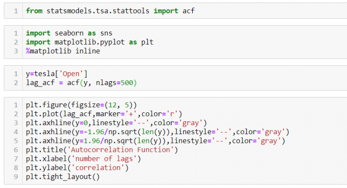
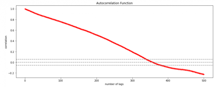
ACF (Auto-correlation function) :- This function calculates the auto-correlation of the complete data on the basis of lagged values which when plotted helps us choose the value of q that is to be considered to find the value of Y_t. In simple words how many years residual can help us predict the value of Y_t can obtained with the help of ACF, if the value of correlation is above a certain point then that amount of lagged values can be used to predict Y_t.

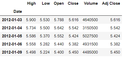
Using the stock price of tesla between the years 2012 and 2017 we can use the .acf() method in python to obtain the value of p.

.DataReader() method is used to extract the data from web.

The above graph shows that beyond the lag 350 the correlation moved towards 0 and then negative.

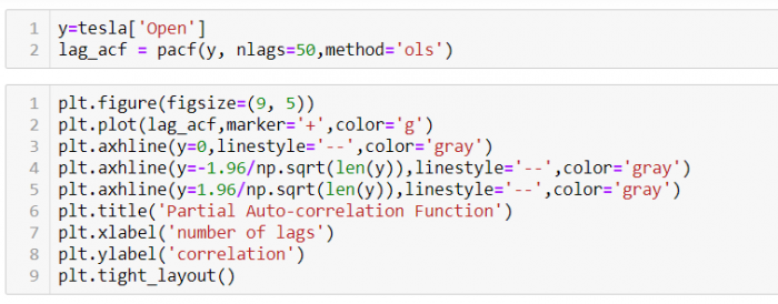
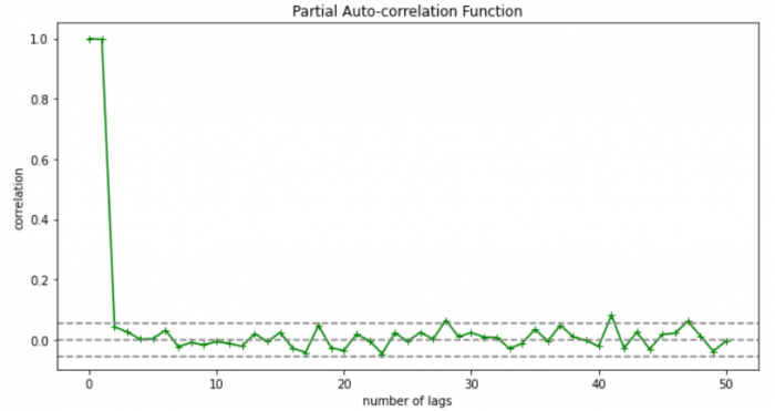
PACF (Partial auto-correlation function) :- Pacf helps find the direct effect of the past lag by removing the residual effect of the lags in between. Pacf helps in obtaining the value of AR where as acf helps in obtaining the value of MA i.e. q. Both the methods together can be use find the optimum value of p and q in a time series data set.

Lets check out how to apply pacf in python.

As you can see in the above graph after the second lag the line moved within the confidence band therefore the value of p will be 2.

So, with that we come to the end of the discussion on the ARMA Model. Hopefully it helped you understand the topic, for more information you can also watch the video tutorial attached down this blog. The blog is designed and prepared by Niharika Rai, Analytics Consultant, DexLab Analytics DexLab Analytics offers machine learning courses in Gurgaon. To keep on learning more, follow DexLab Analytics blog.

Autocorrelation- Time Series – Part 3

Posted on January 22, 2021February 13, 2021 by Dexlab

Autocorrelation is a special case of correlation. It refers to the relationship between successive values of the same variables .For example if an individual with a consumption pattern:-

spends too much in period 1 then he will try to compensate that in period 2 by spending less than usual. This would mean that Ut is correlated with Ut+1 . If it is plotted the graph will appear as follows :

Positive Autocorrelation : When the previous year’s error effects the current year’s error in such a way that when a graph is plotted the line moves in the upward direction or when the error of the time t-1 carries over into a positive error in the following period it is called a positive autocorrelation.
Negative Autocorrelation : When the previous year’s error effects the current year’s error in such a way that when a graph is plotted the line moves in the downward direction or when the error of the time t-1 carries over into a negative error in the following period it is called a negative autocorrelation.

Now there are two ways of detecting the presence of autocorrelation
By plotting a scatter plot of the estimated residual (ei) against one another i.e. present value of residuals are plotted against its own past value.

If most of the points fall in the 1st and the 3rd quadrants , autocorrelation will be positive since the products are positive.

If most of the points fall in the 2nd and 4th quadrant , the autocorrelation will be negative, because the products are negative.
By plotting ei against time : The successive values of ei are plotted against time would indicate the possible presence of autocorrelation .If e’s in successive time show a regular time pattern, then there is autocorrelation in the function. The autocorrelation is said to be negative if successive values of ei changes sign frequently.
First Order of Autocorrelation (AR-1)
When t-1 time period’s error affects the error of time period t (current time period), then it is called first order of autocorrelation.
AR-1 coefficient p takes values between +1 and -1
The size of this coefficient p determines the strength of autocorrelation.
A positive value of p indicates a positive autocorrelation.
A negative value of p indicates a negative autocorrelation
In case if p = 0, then this indicates there is no autocorrelation.
To explain the error term in any particular period t, we use the following formula:-

Where Vt= a random term which fulfills all the usual assumptions of OLS
How to find the value of p?

One can estimate the value of ρ by applying the following formula :-

Time Series Analysis & Modelling with Python (Part II) – Data Smoothing

Posted on January 20, 2021January 20, 2021 by Dexlab

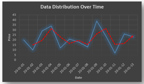
Data Smoothing is done to better understand the hidden patterns in the data. In the non- stationary processes, it is very hard to forecast the data as the variance over a period of time changes, therefore data smoothing techniques are used to smooth out the irregular roughness to see a clearer signal.

In this segment we will be discussing two of the most important data smoothing techniques :-

Moving average smoothing
Exponential smoothing

Moving average smoothing

Moving average is a technique where subsets of original data are created and then average of each subset is taken to smooth out the data and find the value in between each subset which better helps to see the trend over a period of time.

Lets take an example to better understand the problem.

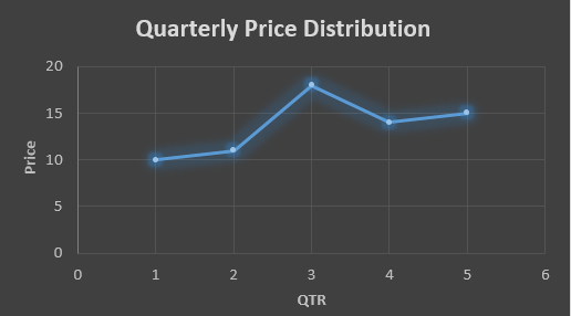
Suppose that we have a data of price observed over a period of time and it is a non-stationary data so that the tend is hard to recognize.

QTR (quarter)	Price
1	10
2	11
3	18
4	14
5	15
6	?

In the above data we don’t know the value of the 6^th quarter.

….fig (1)

The plot above shows that there is no trend the data is following so to better understand the pattern we calculate the moving average over three quarter at a time so that we get in between values as well as we get the missing value of the 6^th quarter.

To find the missing value of 6^th quarter we will use previous three quarter’s data i.e.

MAS = = 15.7

QTR (quarter)	Price
1	10
2	11
3	18
4	14
5	15
6	15.7

MAS = = 13

MAS = = 14.33

QTR (quarter)	Price	MAS (Price)
1	10	10
2	11	11
3	18	18
4	14	13
5	15	14.33
6	15.7	15.7

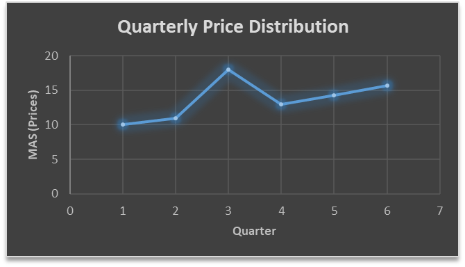
….. fig (2)

In the above graph we can see that after 3^rd quarter there is an upward sloping trend in the data.

Exponential Data Smoothing

In this method a larger weight ( ) which lies between 0 & 1 is given to the most recent observations and as the observation grows more distant the weight decreases exponentially.

The weights are decided on the basis how the data is, in case the data has low movement then we will choose the value of closer to 0 and in case the data has a lot more randomness then in that case we would like to choose the value of closer to 1.

EMA= F_t= F_t-1 + (A_t-1 – F_t-1)

Now lets see a practical example.

For this example we will be taking = 0.5

Taking the same data……

QTR (quarter)	Price (A_t)	EMS Price(F_t)
1	10	10
2	11	?
3	18	?
4	14	?
5	15	?
6	?	?

To find the value of yellow cell we need to find out the value of all the blue cells and since we do not have the initial value of F₁ we will use the value of A_1.Now lets do the calculation:-

F₂=10+0.5(10 – 10) = 10

F₃=10+0.5(11 – 10) = 10.5

F₄=10.5+0.5(18 – 10.5) = 14.25

F₅=14.25+0.5(14 – 14.25) = 14.13

F₆=14.13+0.5(15 – 14.13)= 14.56

QTR (quarter)	Price (A_t)	EMS Price(F_t)
1	10	10
2	11	10
3	18	10.5
4	14	14.25
5	15	14.13
6	14.56	14.56

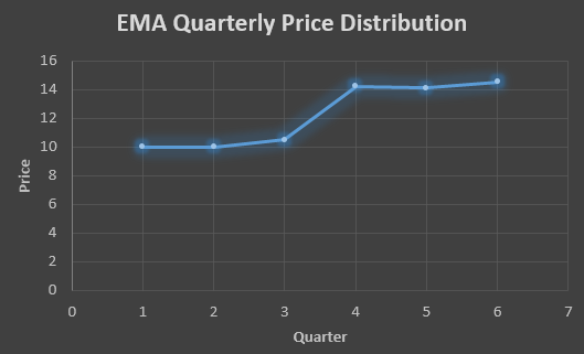
In the above graph we see that there is a trend now where the data is moving in the upward direction.

So, with that we come to the end of the discussion on the Data smoothing method. Hopefully it helped you understand the topic, for more information you can also watch the video tutorial attached down this blog. The blog is designed and prepared by Niharika Rai, Analytics Consultant, DexLab Analytics DexLab Analytics offers machine learning courses in Gurgaon. To keep on learning more, follow DexLab Analytics blog.

Time Series Analysis Part I

Posted on January 18, 2021January 18, 2021 by Dexlab

A time series is a sequence of numerical data in which each item is associated with a particular instant in time. Many sets of data appear as time series: a monthly sequence of the quantity of goods shipped from a factory, a weekly series of the number of road accidents, daily rainfall amounts, hourly observations made on the yield of a chemical process, and so on. Examples of time series abound in such fields as economics, business, engineering, the natural sciences (especially geophysics and meteorology), and the social sciences.

Univariate time series analysis- When we have a single sequence of data observed over time then it is called univariate time series analysis.
Multivariate time series analysis – When we have several sets of data for the same sequence of time periods to observe then it is called multivariate time series analysis.

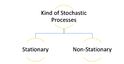
The data used in time series analysis is a random variable (Yt) where t is denoted as time and such a collection of random variables ordered in time is called random or stochastic process.

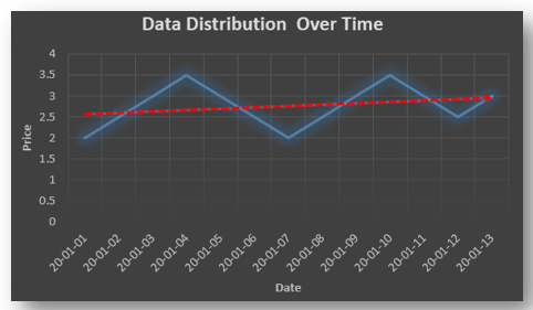
Stationary: A time series is said to be stationary when all the moments of its probability distribution i.e. mean, variance , covariance etc. are invariant over time. It becomes quite easy forecast data in this kind of situation as the hidden patterns are recognizable which make predictions easy.

Non-stationary: A non-stationary time series will have a time varying mean or time varying variance or both, which makes it impossible to generalize the time series over other time periods.

Non stationary processes can further be explained with the help of a term called Random walk models. This term or theory usually is used in stock market which assumes that stock prices are independent of each other over time. Now there are two types of random walks:
Random walk with drift : When the observation that is to be predicted at a time ‘t’ is equal to last period’s value plus a constant or a drift (α) and the residual term (ε). It can be written as
Yt= α + Yt-1 + εt
The equation shows that Yt drifts upwards or downwards depending upon α being positive or negative and the mean and the variance also increases over time.
Random walk without drift: The random walk without a drift model observes that the values to be predicted at time ‘t’ is equal to last past period’s value plus a random shock.
Yt= Yt-1 + εt
Consider that the effect in one unit shock then the process started at some time 0 with a value of Y0
When t=1
Y1= Y0 + ε1
When t=2
Y2= Y1+ ε2= Y0 + ε1+ ε2
In general,
Yt= Y0+∑ εt
In this case as t increases the variance increases indefinitely whereas the mean value of Y is equal to its initial or starting value. Therefore the random walk model without drift is a non-stationary process.

So, with that we come to the end of the discussion on the Time Series. Hopefully it helped you understand time Series, for more information you can also watch the video tutorial attached down this blog. DexLab Analytics offers machine learning courses in delhi. To keep on learning more, follow DexLab Analytics blog.

Customer Analytics: A Basic Introduction

Posted on June 10, 2019June 22, 2019 by Dexlab

Customer Analytics: A Basic Introduction

Customer Analytics is today’s hottest kid on the block, especially for executives. In simple terms, customer analytics is the process of analyzing and evaluating a flood of data that is being collected every day from every possible and probable customer standpoint. This customer data is then used in building superior predictive models to ascertain who the best customers for the retailer are, where he can find this kind of customer base and the value-potential these customers possess – either in terms of visits or dollars.

Customer data provides valuable and actionable insights that help retailers in executing their future marketing and real estate strategies. Put simply, it basically uses the past to predict the future.

Inadequate Customer Data: The Problem

No wonder, Customer Analytics is indeed a wonderful tool yet it’s not as simple as it sounds. Basically, collecting and determining data is an expensive affair as well as time-consuming. However, it is an absolute necessity. If not this, the retailers won’t be able to realize the potentials of customer analytics to the fullest.

However, most of the retailers, at least 60% of the lot don’t have access to data or they possess unreliable data. Generally speaking, an average company’s data is nearly 55% accurate and 14 months old, which makes the data fundamentally useless.

Faulty data skews customer profiles – resulting in lost opportunities, escalating costs, poor use of analytic solutions, dwindling numbers of customers – effectively costing retailers $700 billion annually.

Interestingly, the companies that have mastered the art of Customer Analytics are 7.4 times more likely to outdo their rivals in terms of sales, 6.5 times more likely to retain existing customers and approximately 19 times more likely to hit above-average profitability.

Why Use Customer Analytics?

While there are retailers who have just grazed the layers of customer insights, you will find another set of retailers who are successfully utilizing the treasure trove of customer data merging analytics into it and identifying crucial information that leads to streamlining operations, accelerating productivity, personalizing marketing initiatives in accordance to both current and potential customers. This yields better profitability and detects locations where retailers can open new shops and target new customers.

With such intense market competition, retailers need to outnumber their tailing rivals and for that, they have to leverage the power of customer analytics. Instead of being an option, it has now become a necessity. So, say thanks to Customer Analytics, because of it, retailers are in a position to greatly enhance their potentials to target the right customers at the right time in the right place and in the most effective way.

If you are interested in customer marketing analytics courses in Delhi, feel free to reach us at DexLab Analytics. We offer excellent marketing analytics certification courses to the interested candidates at amazing prices! Contact us now.

The blog has been sourced from ― www.buxtonco.com/blog/what-is-customer-analytics

Interested in a career in Data Analyst?
To learn more about Data Analyst with Advanced excel course – Enrol Now.
To learn more about Data Analyst with R Course – Enrol Now.
To learn more about Big Data Course – Enrol Now.
To learn more about Machine Learning Using Python and Spark – Enrol Now.
To learn more about Data Analyst with SAS Course – Enrol Now.
To learn more about Data Analyst with Apache Spark Course – Enrol Now.
To learn more about Data Analyst with Market Risk Analytics and Modelling Course – Enrol Now.

Digital Transformation Calls for Wider Security Transformation!

Posted on October 25, 2018October 25, 2018 by Dexlab

Digital Transformation Calls for Wider Security Transformation!

Going Digital is the buzzword – conventional businesses are getting transformed, thanks to digital bandwagon! Each day, it’s developing some new ways to engage clients, associate with partners and strike better operational efficiencies. Today’s business houses are using digital power to enhance revenue and reduce cost, and we can’t agree more.

Digital business is generally the implementation of digital technologies to support business models through user behavior evolution and considerable regulation support. For an instance, let’s look at Uber:

New Technology – Transportation technology platform
Business Model – Driver-partners and riders model
User Behavior Norm – Acceptance of non-traditional transportation method
Regulation Support – Cities and countries modify regulation to strengthen models

Today, cyber security and technology risk-management are treasure keys to future business growth and prosperity – security industry has evolved a lot over the years in terms of risk mitigation measures. Digital transformation has made way for security transformation, and in this regard, below we’ve whittled down the elements used for security transformation:

Digital Technologies – Smart watches, smart cars, health bands, voice assistants and smart home devices are some of the latest digital technologies clogging the present industry. These devices are to be supported by robust application platforms using AI, Machine Learning and Big Data.

Business Models – Risk management techniques are perfect for determining information risks emanating from business processes. In digital businesses, dynamic processes are common and evolving. Traditional risk models can’t handle them.

Evolving User Behaviors – Consumers are king in the digital world. The users are empowered with tools to make their own choices. On the contrary, traditional security processes used to treat users as weak links.

Regulation Support – To manage risk, security and privacy, regulations around the globe are changing and control standards are being updated or modified. For effective adaptability with the relevant changes, compliance assurance and sustenance need to be modified.

A Few Fundamental Design Principles for Control Framework for Security Transformation

Business Accelerator – Only security is not just good enough for smooth digital transformation. Security has to take the role of an accelerator since the fundamental premise of going digital is to be fast in the market and enhance customer satisfaction.

Example – Biometric Authentic – it improves user speed and experience.

Technology Changes and Agile Design – The stream of technology is evolving – AI, ML, Blockchain, Virtual Reality, Internet of Things, etc. – every domain of technology is undergoing a robust transformation. Therefore, security controls have to be adaptable and agile in design.

Customer-oriented – Known to all, customers are the most important element in digital business. In the new digitized world, users are the ones who decide. Two-decade ago rule, ‘deny all, permit some’ is now changed into ‘permit all, deny some’ rule – and we are truly excited!

Automate and Digitize – It’s time security goes digital – automation is the key.

In the near future, risk management through security transformation is going to be the utmost priority for all risk managers –if you are interested in Market Risk Analytics, drop by DexLab Analytics. They are the best in town for recognized and reputable Value at Risk Model online training. For more, check out their official website.

The blog has been sourced from ― www.forbes.com/sites/forbestechcouncil/2018/09/27/the-digital-transformation-demands-large-scale-security-transformation/#64df7fc41892

Interested in a career in Data Analyst?
To learn more about Data Analyst with Advanced excel course – Enrol Now.
To learn more about Data Analyst with R Course – Enrol Now.
To learn more about Big Data Course – Enrol Now.
To learn more about Machine Learning Using Python and Spark – Enrol Now.
To learn more about Data Analyst with SAS Course – Enrol Now.
To learn more about Data Analyst with Apache Spark Course – Enrol Now.
To learn more about Data Analyst with Market Risk Analytics and Modelling Course – Enrol Now.

Risk Analytics: How to Frame Smarter Insights with Organizational Data

Posted on April 2, 2018April 2, 2018 by Dexlab

Companies are launching cloud-based data analytics solutions with an aim to aid banks improve and manage their risk efficiently and streamline other activities in the most cost-effective ways.

Risk analysis is a major constituent of banking circle. Analytics-intensive operations are being run in almost all banking institutions, including cyber-security, online data theft and third-party management. The concept of risk is not something new. For years, it has been the key responsibility of C-suite professionals, but the extravagant amount of awareness and recognition associated with risk analytics was missing then. Also, the regulatory and economic landscape of the world is changing and becoming more intense – hence, risks need to be managed adequately. The executive teams should make risk analytics their topmost agenda for better organization functioning.

Why risk analytics?

The first and foremost reason to incorporate risk analytics is to measure, quantify and forecast risk with amped certainty. Analytics help in developing a baseline for risk assessment in an organization by working on several dimensions of risk and pulling them in a single unified system for better results.

What are the potential benefits of risk analytics?

Risk analytics help in turning guesswork into meaningful insights by using a number of tools and techniques to draw perspectives, determine calculable scenarios and predict likely-to-happen events.
An organization stay exposed to risk. Why? Because of a pool of structured and unstructured data, including social media, blogs, websites available on both internal and external platforms. With risk analytics, you can integrate all these data into a single perspective offering actionable insights.
Risk is a largely encompassing concept, spilling across several domains of organizational structure that at times it can really be hard to know how to manage risk and pull out meaningful insights. In such situations, risk analytics play a pivotal role in ensuring organizations develop foresight for potential risks and provide answers to difficult questions so as to create a pathway for action.

Things to do now:

Ask the right questions

Analytics means research. It ushers you to ask questions and dig deeper into risk-related stuffs. But framing random questions don’t help. To have a real impact, conjure up a handful of questions that hits the real topic.

Understand interdependencies

Risk pierces into organizational boundaries. And analytics work by offering cross-enterprise insights, by inferring conclusions throughout the business. That makes it effective to tackle far-reaching issues.

Streamline productive programs

Analytics help decision-makers introspect and evaluate risks, as well as rewards – related to operational and strategic decisions. Adding insights into pre-determined actions to determine and curb risks yield sustainable value for the program, which in the end improves overall program performance.

In the end, risk analytics seem to be quite a daunting subject to take up, but the truth is, some organizations are really doing well in managing their risks. If you are frustrated somehow and this whole concept of risk analytics baffles you more, take up SAS risk management certification. DexLab Analytics, a premier market risk training institute offers incredible market risk courses for data-hungry aspirants.

The article has been sourced from – https://www2.deloitte.com/content/dam/Deloitte/global/Documents/Deloitte-Analytics/dttl-analytics-us-da-oriskanalytics3minguide.pdf

Interested in a career in Data Analyst?
To learn more about Machine Learning Using Python and Spark – click here.
To learn more about Data Analyst with Advanced excel course – click here.
To learn more about Data Analyst with SAS Course – click here.
To learn more about Data Analyst with R Course – click here.
To learn more about Big Data Course – click here.

Quantum Computing Going Commercial: IBM and Google Leading the Trail

Posted on March 22, 2018March 22, 2018 by Dexlab

Quantum computing is all set to make a debut in the commercial world – tech bigwigs, like IBM and Google are making an attempt to commercialize quantum computing. Julian Kelly, a top notch research scientist at Google’s Quantum AI Lab announced with a joint collaboration with Bristlecone, a quantum processor that offers a testbed for various research activities on quantum technology and machine learning, quantum supremacy can be achieved and this could be a great stepping stone for building larger scale quantum computers.

After Google, IBM is also making significant progress in commercializing quantum computing technology by taking it to the cloud in 2016 with a 5 qubit quantum computer. Also, last year, November they raised the bar by declaring that they are going to launch third generation quantum computer equipped with a 50 quibit prototype, but they were not sure if it will be launched on commercial platforms, as well. However, they created another 20 qubit system available on its cloud computing platform.

Reasons Behind Making Quantum Computing Commercialized:

Might lead to fourth industrial revolution

Quantum computing has seeped in to an engineering development phase from just a mere theoretical research – with significant technological power and constant R&D efforts it can develop the ability to trigger a fourth industrial revolution.

Beyond classic computing technology

Areas where conventional computers fail to work, quantum computing will instill a profound impact – such as in industrial processes where innovative steps in machine learning or novel cryptography are involved.

Higher revenue

Revenues from quantum computing are expected to increase from US$1.9 billion in 2023 to US$8.0 billion by 2027 – as forecasted by Communications Industry Researchers (CIR).

Market expansion

The scopes of quantum computing have broadened beyond expectations – it has expanded to drug discovery, health care, power and energy, financial services and aerospace industry.

From cloud to on-premise quantum technology

To incorporate quantum computing into the heart of the business operations’ computing strategy, the companies are contemplating to add a new stream of revenue by implementing quantum computing via cloud. In the future, it’s expected to see a rise in on-premise quantum computing – because the technology is already gaining a lot of accolades.

Better growth forecasts

In the current scenario, the quantum enterprise market is still at a nascent stage with a large user base in the R&D space. But by 2024, it has been forecasted that this share would be somewhere around 30% and the powerful revenue drivers will be industries, like defense, banking, aerospace, pharmaceutical and chemical.

IBM or Google? Who is a clear winner?

In the race to win quantum supremacy, IBM is a sure winner and has made stunning progress in this arena, even though it is receiving stiff competition by Google recently. Google’s new quantum processor Bristlecone has the ability to become a “compelling proof-of-principle for building larger scale quantum computers”. For this, Julian Kelly suggested, “operating a device such as Bristlecone at low system error requires harmony between a full stack of technology ranging from software and control electronics to the processor itself. Getting this right requires careful systems engineering over several iterations.”

As last notes, quantum computing has come out from being a fundamental scientific research to a structural engineering concept. Follow a full-stack approach, coupled with rapid testing and innovative practices and establish winning control over this future tool of success.

In this endeavor, DexLab Analytics can for sure be of help! Their business analytics certification online courses are mindblowing. They also offer machine learning using python courses and market risk training – all of them are student-friendly and prepared after thorough research and fact-finding.

The article has been sourced from – https://analyticsindiamag.com/why-are-big-tech-giants-like-google-ibm-rushing-to-commercialize-quantum-computing

Interested in a career in Data Analyst?
To learn more about Machine Learning Using Python and Spark – click here.
To learn more about Data Analyst with Advanced excel course – click here.
To learn more about Data Analyst with SAS Course – click here.
To learn more about Data Analyst with R Course – click here.
To learn more about Big Data Course – click here.

Call us to know more

Gurgaon

Kolkata