Machine Learning Training Archives - Page 3 of 18 - DexLab Analytics | Big Data Hadoop SAS R Analytics Predictive Modeling & Excel VBA

Gradient Boosting In scikit-learn 0.22 For Handling Missing Values

Posted on August 10, 2020August 10, 2020 by Dexlab

A new tutorial session regarding the scikit-learn 0.22 is here and our sole focus is going to be updating your knowledge regarding the new features that have been added to this library. For this particular session we have decided to introduce you to the concept of gradient boosting that can handle the missing values. This concept is being introduced to clear out a previous misconception regarding the functioning of gradient boosting for this particular purpose.

The earlier notion surrounding GBM or, the gradient boosting algorithm in scikit-learn, was that it was unable to handle the missing values. In this tutorial we want to clarify that misconception, because, contrary to the notion XGBoost library or, XGB library is perfectly capable of handling the missing value analysis. It has been found that XGB library performs better than the normal method taken to find the missing values.

Now getting back to the scikit-learn 0.22 way of solving the issue of missing values. There has been an enhancement in the algorithm gradient boosting due to which you no longer have to handle the missing values because it will handle it of itself.

So take a look at how the concept of native support for missing values for gradient boosting works.

The ensemble algorithm, ensemble.HistGradientBoostingClassifier and ensemble.HistGradientBoostingRegressor, both classification regression now have the power of native support for missing values or, (NaNs). This is indicative of the fact that there is no need now for imputing data during training or predicting.

To gain an insight into how you perform this you need to follow the complete code sheet that you can find here

Now, as you go through the code you will find the word enable, which might surprise you and make you question why it says enable here? Well, this is because it is still being developed.

So, basically all of the algorithms in the scikit-learn 0.22 that are under development process have to run an extra line of code that goes like enable_hist_gradient_boosting. After further development there won’t be any need of that.

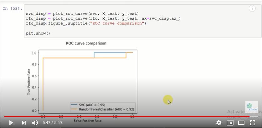
The video attached below will further explain how the algorithm works.

There will be more informative tutorial sessions like this, so to stay updated keep following the DexLab Analytics blog.

Watch the video here.

Machine Learning Tips From Amazon Web Services: What Are The Key Takeaways?

Posted on July 10, 2020July 10, 2020 by Dexlab

Machine learning is a subset of Artificial Intelligence, or, AI which draws from its past experiences to predict future action and act on it. The growing demand for Machine Learning course in Gurgaon, is a clear pointer to the growth the field is experiencing.

If you have been on Youtube frequently then you would certainly have noticed, how it recognizes the choices you made during your last visit and it suggests results based on those past interactions.

The world of machine learning is way past its nascent stage and has found several avenues where its application has become manifold over the years. From predictive analysis to pattern recognition systems, Machine learning is being put to use for finding an array of solutions.

AWS has been a pioneer in the field as it embraced the technology almost 20 years back, recognizing its potential growth across all business verticals.

At a recently held online tech conference, vice president of Amazon AI shared his concerns and ideas regarding the journey of ML while pointing out the hurdles still in the way and which need to be addressed. Here are the key takeaways from the discussion

Growing need for Machine learning

Amazon was quick to realize a crucial fact in the very beginning that consumer experience is a crucial aspect of business which needs to get better with the application of ML.

Despite the impressive trajectory of machine learning and its growing application across different fields there are still issues which pose serious challenge. There are certain issues which if tackled properly would pave the way for a smarter future for all.

Get your data together

Businesses intent on building a machine learning strategy need to understand that they are missing a vital component of the model which is the data itself. Setting out business objectives is not enough; machine learning model is basically built upon data. You need to feed the model data, accumulated over a period of time which it could analyze and to predict future action.

Clarity regarding machine learning application

It is understood that you need to apply machine learning in order to find solutions, to do that you need to identify that particular area of your business where you need the solution. Once you have done that, you need clarity regarding data backup, applicability and impact on business. Swami Sivasubramaniam, vice president of Amazon AI at Amazon Web Services referred to these aspects as “three dimensions”.

Another point he stressed was regarding a collaboration between domain experts and machine learning teams.

Dearth of skill

Although there has been a quantum growth in the application of machine learning, there is a significant lack of trained personnel for handling machine learning models. Undergoing a Machine Learning course in Gurgaon, could bridge the skill gap.

Since, this sector is poised to grow, people willing to make a career should consider undergoing training.

In fact, organizations looking to implement machine learning model, should send their employees for corporate training programs offered at a premier MIS Training Institute in Delhi NCR.

Avoid undifferentiated heavy lifting

Most companies tend to shift their focus from the job at hand and according to Sivasubramaniam, starts dealing with issues like “server hosting, bandwidth management, contract negotiation…”, when they should only be concerned with making the model work for their business model and should look for cloud-based solutions for handling the rest of the issues.

Addressing these issues would only pave the way towards a brighter future where Machine learning would become an integral part of every business model.

Source: https://searchenterpriseai.techtarget.com/feature/How-to-build-a-machine-learning-model-in-7-steps

KNN Imputer – Release Highlights for Scikit-learn 0.22

Posted on July 1, 2020August 10, 2020 by Dexlab

Today we are going to learn about the new feature of Scikit-learn version 0.22 called KNN Imputation. This feature now enables us to support imputation for completing missing values using k-Nearest Neighbours (KNN). To track our tutorials on other new releases from scikit-learn, read our blog here and here.

Introduction

Each sample’s missing values are imputed using the mean value from nearest neighbours found in the training set. Two samples are close if the features that are neither missing are close. By default, a Euclidean distance metric that supports missing values, nan_euclidean_distances, is used to find the nearest neighbours.

Input and Output

So, what we do first is to import libraries like NumPy and run them. Then we create as many rows as we wish to. Then we run the function KNN Imputer and we can decide how many neighbours we want. We first, as is the procedure to use scikit-learn goes, create an object and then run it. Then we can directly put the input values in imputer.fit_transform and get the output values in the form of patterns detected in the input values.

The code sheet for this tutorial is provided in a Github repository here

For more on this do watch the video attached herewith. This tutorial was brought to you by DexLab Analytics. DexLab Analytics is a premiere Machine Learning institute in Gurgaon.

Watch the video here.

Machine Learning Algorithms – With Python (Part II)

Posted on June 22, 2020June 22, 2020 by Dexlab

In the first part of this blog, we covered Parametric and Non-Parametric Machine Learning algorithms and Supervised and Unsupervised Machine Learning Algorithms. If you haven’t gone through it yet, check it out here: dexlabanalytics.com/blog/machine-learning-algorithms-with-python-part-i

In this blog we are going learn about Semi Supervised Machine Learning algorithms.

What are Semi Supervised ML algorithms?

Those algorithms in which only half of the historical data’s target data has been specified are called semi-supervised algorithms. The way to go about solving this is by making a model on the basis of the portion of historical data that has the target specified and then apply this model to the rest of the data to predict the outcomes. Now, combine the two sets of data, get the target variable and make a model on the basis of this target variable.

New Nomenclature

In the equation Y= B0 + B1X, Y is called the Target Variable while in statistics it is called the Dependent Variable. And X is called Features or Attributes whereas in statistics it is called Independent Variable. B0 and B1 are called Weights while in statistics they are called Coefficients (Intercept and Slope, respectively).

In the equation Ÿ – Y = error, the error in statistics is called Residual but in Machine Learning it is called Cost Function. And the elements of the historical data set that in statistics are known as Records or Observations, in machine learning are known as Instances.

What is Bias Variance Trade-Off?

In parametric algorithms like linear regressions, several assumptions are made before building a model. These assumptions can be things like having only those inputs that have a relationship with the target variable or the fact that the error should be random. The benefit of this process is the fact that Ÿ or the predicted results are consistent and there is not much variance in them.

Now, if we are to take a Decision Tree or any other non-parametric Machine Learning algorithm, a small change in the data set forces a large variance in the Target variable. But, unlike in parametric ML algorithms, there are no basic assumptions in non-parametric assumptions. So, in such a case, the error or mean square error, is a combination of the square of bias and variance.

MSE = Bias2 + Variance

Increasing any one (the square of the bias) will lead to a decrease in the other (variance) and vice versa.

In this case, we need to balance or trade off the two – the square of the bias and the variance.

While the bias cannot be changed much, we can control the variance by increasing or decreasing the parameters of the experiment.

What is Overfitting and Underfitting?

Overfitting is the condition when the accuracy figure of the ‘trained’ data set is larger in number than the accuracy figure of the ‘tested’ unseen data set. This is an undesirable condition. Underfitting is the opposite wherein the accuracy figure of the trained data is lower than that of the tested unseen data. This is also undesirable. What we seek to aim at is an equal accuracy in both the tested and trained models.

To limit Overfitting we must –

Use a resampling technique to estimate model accuracy by repeating experiments with the data and then drawing an average of the accuracy figures.
Hold back a validation data set to test your model on and increase the number of models to experiment on the trained data set.

We would like to conclude out second part of this tutorial here. For more on this, visit the third blog on Machine Learning Algorithms with Python.

(Translated from 28:00 – 1:19:00)

Machine Learning Algorithms – With Python (Part I)

Posted on June 17, 2020June 22, 2020 by Dexlab

Our industry experts introduce beginners to Machine Learning Algorithms with Python. In this blog, we will go through various Machine Learning Algorithms to understand the concepts better. This is the first part of a series.

Machine Learning, a subset of Artificial Intelligence, is a process of data analysis that automates analytical model building. It is a branch of artificial intelligence based on the idea that computing systems can learn from data, identify patterns in them and make intelligent decisions with minimal human intervention.

Parametric and Non-Parametric ML Algorithms

We first divide the mathematical methods for decision making in to sections – parametric and non-parametric algorithms. Parametric has a functional form while non-parametric has no functional form.

Functional form comprises a simple formula like 2+2=4 or Y=F(X). So if you input a value, you are to get a fixed output value. That means, if the data set is changed or being changed, there is not much variation in the results. But in non-parametric algorithms, a small change in data sets can result in a large change in the results.

But we do not desire this. We do not want this massive change in results in investments, for instance. We have various ways to solve this difficulty. For example, in statistics, you must have learnt the Central Limit Theorem – As the number of samples increase, the data will start following the normal distribution.

Here is an experiment on decision making with the help of non-parametric algorithm. We first take a random sample, and we apply an algorithm to it to get a result. We repeat this process several times and get an average of the results. In this way, the variation in our results goes down considerably. We will get a central tendency.

Take for example stock market data where prices are totally random. There is no fixed pattern to it. It is a manmade phenomenon. In the same way, we can make predictions in data sets only when there is a particular pattern. It becomes that much more difficult to make predictions in the absence of a clear pattern. In such a case, we take thousands of samples and work them to get a result before investing. We can use a Decision Tree like Random Forest for this.

Supervised and Unsupervised Algorithms

Now, secondly, we can term ML algorithms as supervised or unsupervised algorithms. Suppose we have data under sub-heads – Name, Age, Gender and Salary and Period of Service. Now, consider the model wherein we are asked to predict the period of service of an employee based on data provided under the rest of the sub-heads based on existing employee data.

Now, in this example, the period of service is the Target. The data sets on the basis of which the prediction will be made – Name, Age, Gender, Salary – is the Input. In such a model, where the target variable is specified, we term it as supervised machine learning algorithm. We do this according to a formula – Y=B0 + B1X1.

In unsupervised learning, the target variable is not provided and all we can do is divide the historical data in clusters. For example, Google Translate runs on a supervised model as do chatbots. Data is not only the new oil, it is everything. And there will come a time of data colonisation whereby the organisation with the best data will rule. The better the date, the better our ML models. Who has the best data sets in the world? Google and Amazon, among others, do.

So this is it, about supervised and unsupervised machine learning. For more on this, do watch our intensive video tutorial on ML algorithms.

(Translated till first 28:00 minutes)

This is the first blog of the series, stay tuned with Dexlab Analytics to read through the whole video we’ll covering in our upcoming blogs!

ROC-AUC-for-Multi-Class-Classification-Release Highlights for Scikit-learn 0.22

Posted on June 10, 2020August 10, 2020 by Dexlab

Today we are going to learn about the new releases from Scikit-learn version 0.22, a machine learning library in Python. We, through this video tutorial, aim to learn about the much talked about new release wherein ROC-AUC curve supports Multi Class Classification. Prior to this version, Scikit-learn did not have a function to plot the ROC curve.

To access our previous tutorial on the plotting of the ROC curve, click here.

The ROC-AUC score function can also be used in multi-class classification. Two averaging strategies are currently supported: the one-vs-one (OvO) algorithm computes the average of the pairwise ROC AUC scores and the one-vs-rest (OvR) algorithm computes the average of the ROC AUC scores for each class against all other classes.

In both cases, the multiclass ROC AUC scores are computed from probability estimates that a sample belongs to a particular class according to the model. The OvO and OvR algorithms support weighting uniformly (average=’macro’) and weighting by prevalence (average=’weighted’).

To begin with, we import multi classification, SVC and roc_auc_score. Then we specify the number of classes we want in the multi-classification function. Then we apply the SVC function and finally the roc_auc_score one. This function will give us the probable prediction for all the classes and we will then choose the one that has the highest probability. When we run it we get a ROC_AUC score of 0.99.

The code sheet is provided in a Github repository here.

For more on this do watch the video attached herewith. This tutorial was brought to you by DexLab Analytics. DexLab Analytics is a premiere Machine Learning institute in Gurgaon.

Watch the video here.

ROC-Curve-New-Plotting-API-Release Highlights for Scikit-learn 0.22

Posted on June 3, 2020August 10, 2020 by Dexlab

Today we are going to learn about the new releases from Scikit-learn version 0.22, a machine learning library in Python. We, through this video tutorial, aim to learn about the much talked about new release called Plotting API. Prior to this version, Scikit-learn did not have a function to plot the ROC curve.

A new plotting API is available for creating visualizations. The new API allows for quickly adjusting the visuals of a plot without involving any recomputation. It is also possible to add different plots to the same figure. In this tutorial we are going to study the plotting of the ROC curve.

The code sheet is provided in a Github repository here.

We will attempt to plot the ROC curve on two different algorithms and compare which one is a better function. First we choose to make a classification data. Then we go on to plot the ROC curve using SVC classifier and then further plot the curve using a random forest classifier.

Fig. 1

Fig. 1

For more on this do watch the video attached herewith. This tutorial was brought to you by DexLab Analytics. DexLab Analytics is a premiere Machine Learning institute in Gurgaon.

How Machine Learning Helped Demystify Locust Breeding Sites

Posted on May 29, 2020May 29, 2020 by Dexlab

Even as the coronavirus pandemic rages on and India is living through a strict lockdown to abate the spread of the novel virus, a disastrous spell of a plague of crop destroying locusts has struck Rajasthan, Gujarat and parts of Madhya Pradesh.

Threatening to balloon into an agrarian crisis, the destruction of crops on this scale is being seen as one “worst in decades”. In fact, such large scale breeding of locusts and an attack by them is the worst in 27 years, government officials said.

In such frightening circumstances, what we can truly bank upon to detect and fight locust attacks is advanced technology like machine learning techniques. This essay aims to demystify how machine learning can be used to detect locust breeding patterns by studying soil moisture through remote sensing.

The Study

Image Source: spiedigitallibrary.org

A study called “Machine learning approach to locate desert locust breeding areas based on ESA CCI soil moisture” shows how researchers have “used two machine learning algorithms (generalized linear model and random forest) to evaluate the link between hopper presences and SM (Soil Moisture) conditions under different time scenarios…It was found that an area becomes suitable for breeding when the minimum SM values are over 0.07 m3 / m3 during 6 days or more. These results demonstrate the possibility to identify breeding areas in Mauritania by means of SM, and the suitability of ESA (European Space Agency) CCI (Climate Change Initiative) SM product to complement or substitute current monitoring techniques based on precipitation datasets.”

The Findings

The study found that “it is widely assumed” that rainfall over 25 mm in two consecutive months is conducive to locust breeding. Likewise, various soil moisture conditions affect breeding patterns greatly. So, the study finds that it is important to have “variable creation as a previous step to modeling”. Different time intervals of locust breeding were tested by the researchers for model creation. Also, different soil moisture values were considered.

Image Source: spiedigitallibrary.org

It was found that the “highest performance was acquired by the RF (Random Forest) algorithm when dividing the whole survey time into ranges of 6 days, and selecting the minimum SM as the variable value.” GLMs of Generalised Linear Models, however, did not work well according to the study.

The applied methodology of machine learning offers promising results to accurately identify breeding areas based on data pertaining to 30 years of SM values. The ESA CCI soil moisture data is one of the most authoritative ones in the world. Thus the researchers who conducted this study are confident that their results signify a breakthrough in locust monitoring technique prevalence in the world.

Conclusion

This study, thus, proposes a machine learning approach based on SM time series “to predict breeding areas, by means of remote sensing”. Artificial Intelligence and Machine Learning will help future researchers and scientists to study and produce better warning systems based on the results of this study. In this study only soil moisture data has been used but more variables like temperatures can also be taken into account to accurately predict breeding grounds in the future.

For more on machine learning applications, do peruse the Dexlab Analytics website today. This article was brought to you by DexLab Analytics, a premier institute offering Machine Learning courses in Delhi.

The blog has been sourced from ― Machine learning approach to locate desert locust breeding areas based on ESA CCI soil moisture

93% Indian Professionals Benefitting From E-Learning During Lockdown: Linkedin

Posted on May 27, 2020May 27, 2020 by Dexlab

The Covid-19 pandemic has struck India like it has scores of countries across the world. As of May 27, over 1,51,000 Indians have been tested positive for the novel virus and over 4000 people have died due to the contagious disease. India has been under lockdown for over two months now in an attempt at abating the spread of the virus due to movement and contact.

With all offices closed and work from home decreed across numerous sectors of the economy, professionals have been forced to adapt to a new mode of work and training. With more time on hand since they are working from home, professionals are upgrading their skills by taking up online training modules and classes. A recent LinkedIn survey throws light on this phenomenon.

LinkedIn’s Work Force Confidence Index

India’s foremost social networking site that helps individuals network with professional peers and find jobs and appointments has conducted a survey called Work Force Confidence Index. As per the survey conducted between April 27 and May 3, “India’s professionals are logging learning hours for not just knowledge acquisition but also to increase productivity. About half of respondents from mid-market firms joined courses that help them manage time better, improve prioritisation or stay organised”.

93% Indian Professionals Benefitting From E-Learning During Lockdown: Linkedin

93% respondents to upskill online in next two weeks

According to LinkedIn News India, 1040 professionals were surveyed by LinkedIn and 93% of them said “their time spent on e-learning will either increase or remain the same over the next two weeks”. Moreover, 60% of the respondents of which 74% were from the engineering domain said e-learning was a conduit to furthering industry knowledge. “Advancing in one’s career was a driver for 57% of all respondents and 3 in 10 active job seekers undertook e-learning to make a career pivot,” said LinkedIn News India.

What respondents learnt

Of the respondents, 45% said they hoped to learn to collaborate with peers through online learning in lockdown. Also, 43% said they wished to learn to manage time and prioritise and stay organised. Moreover, 40% said they hoped to learn something unrelated to work through online platforms. Becoming a leader and managing personal finances were pegged at 37% and 32% respectively by the study as goals and 24% said e-learning could actually lead to a change in career paths for them.

Advantages of e-learning

Travelling to work and back is taxing and time consuming. When you are working from home, you save on energy and time that can be used for something productive like e-learning training modules. They are easy on the pocket, accessible from absolutely anywhere you are and convenient to absorb and retain information and new things learnt. Moreover, there is a large online community to help you out with study material and guidance.

There are many popular e-learning courses in India, especially those around data science and artificial intelligence. DexLab Analytics is a premier credit risk modeling training institute that also trains professionals in artificial intelligence, machine learning and data science. This article was brought to you by DexLab Analytics.

Call us to know more

Gurgaon

+91 852 787 2444 / +91 85271 91444

Kolkata

+91 931 572 5902