Machine Learning course online Archives - DexLab Analytics | Big Data Hadoop SAS R Analytics Predictive Modeling & Excel VBA

MongoDB Basics Part-II

Posted on February 20, 2021 by Dexlab

In our previous blog we discussed about few of the basic functions of MQL like .find() , .count() , .pretty() etc. and in this blog we will continue to do the same. At the end of the blog there is a quiz for you to solve, feel free to test your knowledge and wisdom you have gained so far.

Given below is the list of functions that can be used for data wrangling:-

updateOne() :- This function is used to change the current value of a field in a single document.

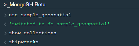
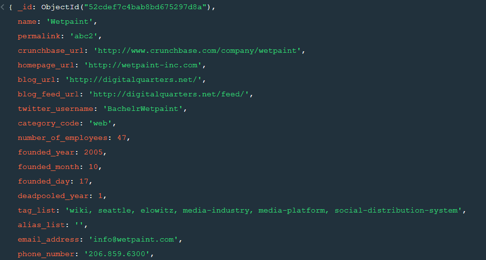
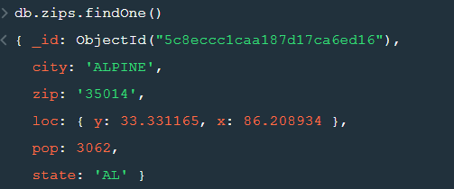
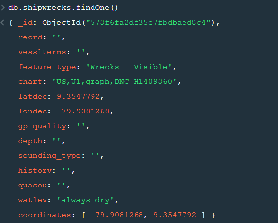
After changing the database to “sample_geospatial” we want to see what the document looks like? So for that we will use .findOne() function.

Now lets update the field value of “recrd” from ‘ ’ to “abc” where the “feature_type” is ‘Wrecks-Visible’.

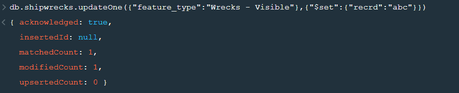
Now within the .updateOne() funtion any thing in the first part of { } is the condition on the basis of which we want to update the given document and the second part is the changes which we want to make. Here we are saying that set the value as “abc” in the “recrd” field . In case you wanted to increase the value by a certain number ( assuming that the value is integer or float) you can use “$inc” instead.

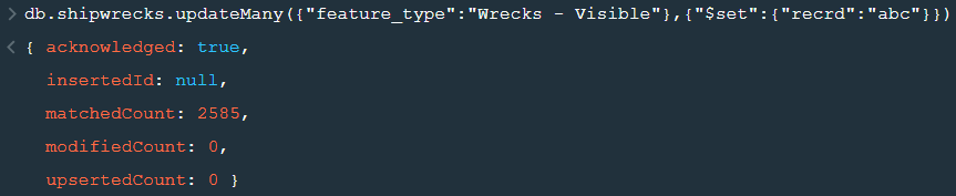
2. updateMany() :- This function updates many documents at once based on the condition provided.

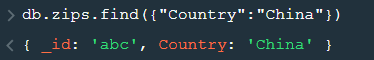
3. deleteOne() & deleteMany() :- These functions are used to delete one or many documents based on the given condition or field.

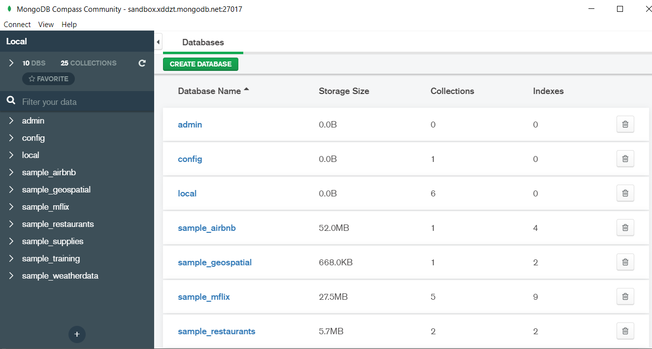
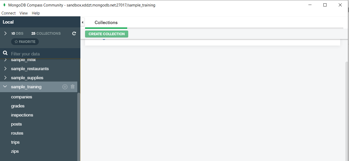
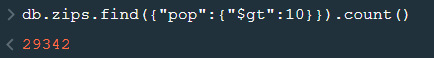
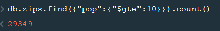
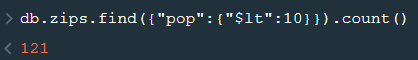
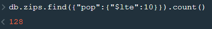
4. Logical Operators :-

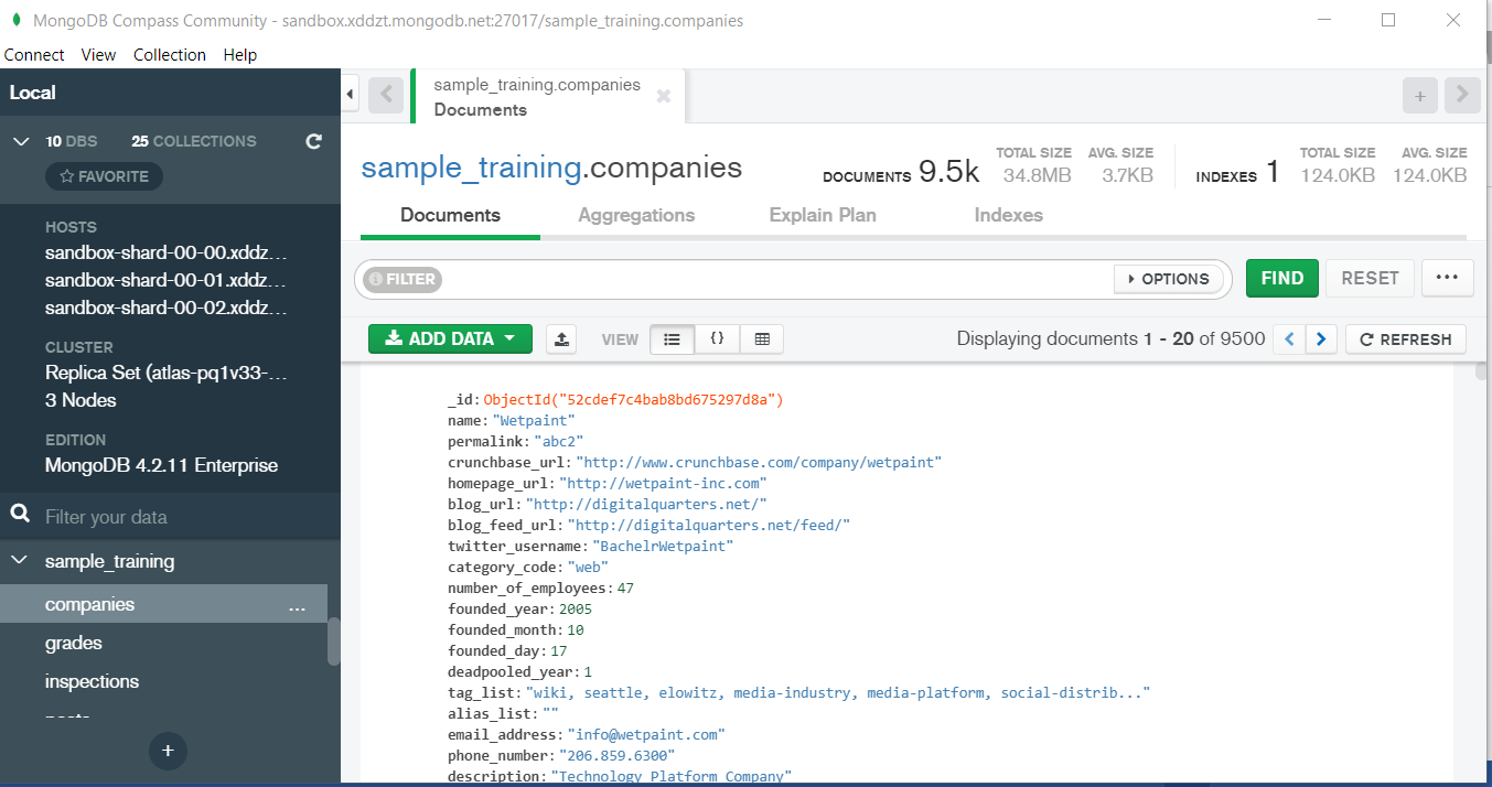
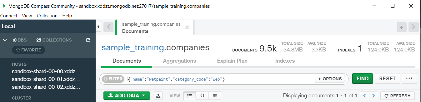
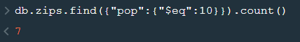
“$and” : It is used to match all the conditions.

“$or” : It is used to match any of the conditions.

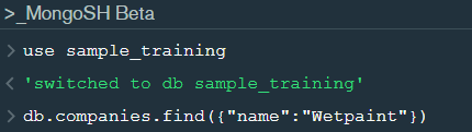
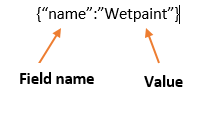
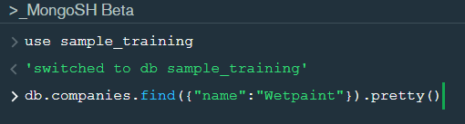
The first code matches both the conditions i.e. name should be “Wetpaint” and “category_code” should be “web”, whereas the second code matches any one of the conditions i.e. either name should be “Wetpaint” or “Facebook”. Try these codes and see the difference by yourself.

So, with that we come to the end of the discussion on the MongoDB Basics. Hopefully it helped you understand the topic, for more information you can also watch the video tutorial attached down this blog. The blog is designed and prepared by Niharika Rai, Analytics Consultant, DexLab Analytics DexLab Analytics offers machine learning courses in Gurgaon. To keep on learning more, follow DexLab Analytics blog.

Introduction to MongoDB

Posted on February 17, 2021February 17, 2021 by Dexlab

MongoDB is a document based database program which was developed by MongoDB Inc. and is licensed under server side public license (SSPL). It can be used across platforms and is a non-relational database also known as NoSQL, where NoSQL means that the data is not stored in the conventional tabular format and is used for unstructured data as compared to SQL and that is the major difference between NoSQL and SQL.
MongoDB stores document in JSON or BSON format. JSON also known as JavaScript Object notation is a format where data is stored in a key value pair or array format which is readable for a normal human being whereas BSON is nothing but the JSON file encoded in the binary format which is quite hard for a human being to understand.
Structure of MongoDB which uses a query language MQL(Mongodb query language):-
Databases:- Databases is a group of collections.
Collections:- Collection is a group fields.
Fields:- Fields are nothing but key value pairs
Just for an example look at the image given below:-

Here I am using MongoDB Compass a tool to connect to Atlas which is a cloud based platform which can help us write our queries and start performing all sort of data extraction and deployment techniques. You can download MongoDB Compass via the given link https://www.mongodb.com/try/download/compass

In the above image in the red box we have our databases and if we click on the “sample_training” database we will see a list of collections similar to the tables in sql.

Now lets write our first query and see what data in “companies” collection looks like but before that select the “companies” collection.

Now in our filter cell we can write the following query:-

In the above query “name” and “category_code” are the key values also known as fields and “Wetpaint” and “web” are the pair values on the basis of which we want to filter the data.
What is cluster and how to create it on Atlas?
MongoDB cluster also know as sharded cluster is created where each collection is divided into shards (small portions of the original data) which is a replica set of the original collection. In case you want to use Atlas there is an unpaid version available with approximately 512 mb space which is free to use. There is a pre-existing cluster in MongoDB named Sandbox , which currently I am using and you can use it too by following the given steps:-
1. Create a free account or sign in using your Google account on
https://www.mongodb.com/cloud/atlas/lp/try2-in?utm_source=google&utm_campaign=gs_apac_india_search_brand_atlas_desktop&utm_term=mongodb%20atlas&utm_medium=cpc_paid_search&utm_ad=e&utm_ad_campaign_id=6501677905&gclid=CjwKCAiAr6-ABhAfEiwADO4sfaMDS6YRyBKaciG97RoCgBimOEq9jU2E5N4Jc4ErkuJXYcVpPd47-xoCkL8QAvD_BwE
2. Click on “Create an Organization”.
3. Write the organization name “MDBU”.
4. Click on “Create Organization”.
5. Click on “New Project”.
6. Name your project M001 and click “Next”.
7. Click on “Build a Cluster”.
8. Click on “Create a Cluster” an option under which free is written.
9. Click on the region closest to you and at the bottom change the name of the cluster to “Sandbox”.
10. Now click on connect and click on “Allow access from anywhere”.
11. Create a Database User and then click on “Create Database User”.
username: m001-student
password: m001-mongodb-basics
12. Click on “Close” and now load your sample as given below :

Loading may take a while….
13. Click on collections once the sample is loaded and now you can start using the filter option in a similar way as in MongoDB Compass
In my next blog I’ll be sharing with you how to connect Atlas with MongoDB Compass and we will also learn few ways in which we can write query using MQL.

So, with that we come to the end of the discussion on the MongoDB. Hopefully it helped you understand the topic, for more information you can also watch the video tutorial attached down this blog. The blog is designed and prepared by Niharika Rai, Analytics Consultant, DexLab Analytics DexLab Analytics offers machine learning courses in Gurgaon. To keep on learning more, follow DexLab Analytics blog.

MongoDB Basics Part-I

Posted on February 12, 2021February 17, 2021 by Dexlab

In this particular blog we will discuss about few of the basic functions of MQL (MongoDB Query Language) and we will also see how to use them? We will be using MongoDB Compass shell (MongoSH Beta) which is available in the latest version of MongoDB Compass.

Connect your Atlas cluster to your MongoDB Compass to get started. Latest version of MongoDB Compass will have this shell, so if you don’t find this shell then please install the latest version for this to work.

Now lets start with the functions.

find() :- You need this function for data extraction in the shell.

In the shell we need to first write the “use database name” code to access the database then use .find() to extract data which has name “Wetpaint”

For the above query we get the following result:-

The above result brings us to another function .pretty() .

2. pretty() :- this function helps us see the result more clearly.

Try it yourself to compare the results.

3. count() :- Now lets see how many entries we have by the company name “Wetpaint”.

So we have only one document.

4. Comparison operators :-

“$eq” : Equal to

“$neq”: Not equal to

“$gt”: Greater than

“$gte”: Greater than equal to

“$lt”: Less than

“$lte”: Less than equal to

Lets see how this works.

5. findOne() :- To get a single document from a collection we use this function.

6. insert() :- This is used to insert documents in a collection.

Now lets check if we have been able to insert this document or not.

Notice that a unique id has been added to the document by default. The given id has to be unique or else there will be an error. To provide a user defined id use “_id”.

So, with that we come to the end of the discussion on the MongoDB. Hopefully it helped you understand the topic, for more information you can also watch the video tutorial attached down this blog. The blog is designed and prepared by Niharika Rai, Analytics Consultant, DexLab Analytics DexLab Analytics offers machine learning courses in Gurgaon. To keep on learning more, follow DexLab Analytics blog.

ARIMA (Auto-Regressive Integrated Moving Average)

Posted on January 27, 2021February 13, 2021 by Dexlab

This is another blog added to the series of time series forecasting. In this particular blog I will be discussing about the basic concepts of ARIMA model.

So what is ARIMA?

ARIMA also known as Autoregressive Integrated Moving Average is a time series forecasting model that helps us predict the future values on the basis of the past values. This model predicts the future values on the basis of the data’s own lags and its lagged errors.

When a data does not reflect any seasonal changes and plus it does not have a pattern of random white noise or residual then an ARIMA model can be used for forecasting.

There are three parameters attributed to an ARIMA model p, q and d :-

p :- corresponds to the autoregressive part

q:- corresponds to the moving average part.

d:- corresponds to number of differencing required to make the data stationary.

In our previous blog we have already discussed in detail what is p and q but what we haven’t discussed is what is d and what is the meaning of differencing (a term missing in ARMA model).

Since AR is a linear regression model and works best when the independent variables are not correlated, differencing can be used to make the model stationary which is subtracting the previous value from the current value so that the prediction of any further values can be stabilized . In case the model is already stationary the value of d=0. Therefore “differencing is the minimum number of deductions required to make the model stationary”. The order of d depends on exactly when your model becomes stationary i.e. in case the autocorrelation is positive over 10 lags then we can do further differencing otherwise in case autocorrelation is very negative at the first lag then we have an over-differenced series.

The formula for the ARIMA model would be:-

To check if ARIMA model is suited for our dataset i.e. to check the stationary of the data we will apply Dickey Fuller test and depending on the results we will using differencing.

In my next blog I will be discussing about how to perform time series forecasting using ARIMA model manually and what is Dickey Fuller test and how to apply that, so just keep on following us for more.

So, with that we come to the end of the discussion on the ARIMA Model. Hopefully it helped you understand the topic, for more information you can also watch the video tutorial attached down this blog. The blog is designed and prepared by Niharika Rai, Analytics Consultant, DexLab Analytics DexLab Analytics offers machine learning courses in Gurgaon. To keep on learning more, follow DexLab Analytics blog.

ARMA- Time Series Analysis Part 4

Posted on January 25, 2021February 13, 2021 by Dexlab

ARMA(p,q) model in time series forecasting is a combination of Autoregressive Process also known as AR Process and Moving Average (MA) Process where p corresponds to the autoregressive part and q corresponds to the moving average part.

Autoregressive Process (AR) :- When the value of Y_t in a time series data is regressed over its own past value then it is called an autoregressive process where p is the order of lag into consideration.

Where,

Y_t = observation which we need to find out.

α₁= parameter of an autoregressive model

Y_t-1= observation in the previous period

u_t= error term

The equation above follows the first order of autoregressive process or AR(1) and the value of p is 1. Hence the value of Y_t in the period ‘t’ depends upon its previous year value and a random term.

Moving Average (MA) Process :- When the value of Y_t of order q in a time series data depends on the weighted sum of current and the q recent errors i.e. a linear combination of error terms then it is called a moving average process which can be written as :-

y_t = observation which we need to find out

α= constant term

β_ut-q= error over the period q .

ARMA (Autoregressive Moving Average) Process :-

The above equation shows that value of Y in time period ‘t’ can be derived by taking into consideration the order of lag p which in the above case is 1 i.e. previous year’s observation and the weighted average of the error term over a period of time q which in case of the above equation is 1.

How to decide the value of p and q?

Two of the most important methods to obtain the best possible values of p and q are ACF and PACF plots.

ACF (Auto-correlation function) :- This function calculates the auto-correlation of the complete data on the basis of lagged values which when plotted helps us choose the value of q that is to be considered to find the value of Y_t. In simple words how many years residual can help us predict the value of Y_t can obtained with the help of ACF, if the value of correlation is above a certain point then that amount of lagged values can be used to predict Y_t.

Using the stock price of tesla between the years 2012 and 2017 we can use the .acf() method in python to obtain the value of p.

.DataReader() method is used to extract the data from web.

The above graph shows that beyond the lag 350 the correlation moved towards 0 and then negative.

PACF (Partial auto-correlation function) :- Pacf helps find the direct effect of the past lag by removing the residual effect of the lags in between. Pacf helps in obtaining the value of AR where as acf helps in obtaining the value of MA i.e. q. Both the methods together can be use find the optimum value of p and q in a time series data set.

Lets check out how to apply pacf in python.

As you can see in the above graph after the second lag the line moved within the confidence band therefore the value of p will be 2.

So, with that we come to the end of the discussion on the ARMA Model. Hopefully it helped you understand the topic, for more information you can also watch the video tutorial attached down this blog. The blog is designed and prepared by Niharika Rai, Analytics Consultant, DexLab Analytics DexLab Analytics offers machine learning courses in Gurgaon. To keep on learning more, follow DexLab Analytics blog.

Autocorrelation- Time Series – Part 3

Posted on January 22, 2021February 13, 2021 by Dexlab

Autocorrelation is a special case of correlation. It refers to the relationship between successive values of the same variables .For example if an individual with a consumption pattern:-

spends too much in period 1 then he will try to compensate that in period 2 by spending less than usual. This would mean that Ut is correlated with Ut+1 . If it is plotted the graph will appear as follows :

Positive Autocorrelation : When the previous year’s error effects the current year’s error in such a way that when a graph is plotted the line moves in the upward direction or when the error of the time t-1 carries over into a positive error in the following period it is called a positive autocorrelation.
Negative Autocorrelation : When the previous year’s error effects the current year’s error in such a way that when a graph is plotted the line moves in the downward direction or when the error of the time t-1 carries over into a negative error in the following period it is called a negative autocorrelation.

Now there are two ways of detecting the presence of autocorrelation
By plotting a scatter plot of the estimated residual (ei) against one another i.e. present value of residuals are plotted against its own past value.

If most of the points fall in the 1st and the 3rd quadrants , autocorrelation will be positive since the products are positive.

If most of the points fall in the 2nd and 4th quadrant , the autocorrelation will be negative, because the products are negative.
By plotting ei against time : The successive values of ei are plotted against time would indicate the possible presence of autocorrelation .If e’s in successive time show a regular time pattern, then there is autocorrelation in the function. The autocorrelation is said to be negative if successive values of ei changes sign frequently.
First Order of Autocorrelation (AR-1)
When t-1 time period’s error affects the error of time period t (current time period), then it is called first order of autocorrelation.
AR-1 coefficient p takes values between +1 and -1
The size of this coefficient p determines the strength of autocorrelation.
A positive value of p indicates a positive autocorrelation.
A negative value of p indicates a negative autocorrelation
In case if p = 0, then this indicates there is no autocorrelation.
To explain the error term in any particular period t, we use the following formula:-

Where Vt= a random term which fulfills all the usual assumptions of OLS
How to find the value of p?

One can estimate the value of ρ by applying the following formula :-

Time Series Analysis & Modelling with Python (Part II) – Data Smoothing

Posted on January 20, 2021January 20, 2021 by Dexlab

Data Smoothing is done to better understand the hidden patterns in the data. In the non- stationary processes, it is very hard to forecast the data as the variance over a period of time changes, therefore data smoothing techniques are used to smooth out the irregular roughness to see a clearer signal.

In this segment we will be discussing two of the most important data smoothing techniques :-

Moving average smoothing
Exponential smoothing

Moving average smoothing

Moving average is a technique where subsets of original data are created and then average of each subset is taken to smooth out the data and find the value in between each subset which better helps to see the trend over a period of time.

Lets take an example to better understand the problem.

Suppose that we have a data of price observed over a period of time and it is a non-stationary data so that the tend is hard to recognize.

QTR (quarter)	Price
1	10
2	11
3	18
4	14
5	15
6	?

In the above data we don’t know the value of the 6^th quarter.

….fig (1)

The plot above shows that there is no trend the data is following so to better understand the pattern we calculate the moving average over three quarter at a time so that we get in between values as well as we get the missing value of the 6^th quarter.

To find the missing value of 6^th quarter we will use previous three quarter’s data i.e.

MAS = = 15.7

QTR (quarter)	Price
1	10
2	11
3	18
4	14
5	15
6	15.7

MAS = = 13

MAS = = 14.33

QTR (quarter)	Price	MAS (Price)
1	10	10
2	11	11
3	18	18
4	14	13
5	15	14.33
6	15.7	15.7

….. fig (2)

In the above graph we can see that after 3^rd quarter there is an upward sloping trend in the data.

Exponential Data Smoothing

In this method a larger weight ( ) which lies between 0 & 1 is given to the most recent observations and as the observation grows more distant the weight decreases exponentially.

The weights are decided on the basis how the data is, in case the data has low movement then we will choose the value of closer to 0 and in case the data has a lot more randomness then in that case we would like to choose the value of closer to 1.

EMA= F_t= F_t-1 + (A_t-1 – F_t-1)

Now lets see a practical example.

For this example we will be taking = 0.5

Taking the same data……

QTR (quarter)	Price (A_t)	EMS Price(F_t)
1	10	10
2	11	?
3	18	?
4	14	?
5	15	?
6	?	?

To find the value of yellow cell we need to find out the value of all the blue cells and since we do not have the initial value of F₁ we will use the value of A_1.Now lets do the calculation:-

F₂=10+0.5(10 – 10) = 10

F₃=10+0.5(11 – 10) = 10.5

F₄=10.5+0.5(18 – 10.5) = 14.25

F₅=14.25+0.5(14 – 14.25) = 14.13

F₆=14.13+0.5(15 – 14.13)= 14.56

QTR (quarter)	Price (A_t)	EMS Price(F_t)
1	10	10
2	11	10
3	18	10.5
4	14	14.25
5	15	14.13
6	14.56	14.56

In the above graph we see that there is a trend now where the data is moving in the upward direction.

So, with that we come to the end of the discussion on the Data smoothing method. Hopefully it helped you understand the topic, for more information you can also watch the video tutorial attached down this blog. The blog is designed and prepared by Niharika Rai, Analytics Consultant, DexLab Analytics DexLab Analytics offers machine learning courses in Gurgaon. To keep on learning more, follow DexLab Analytics blog.

Time Series Analysis Part I

Posted on January 18, 2021January 18, 2021 by Dexlab

A time series is a sequence of numerical data in which each item is associated with a particular instant in time. Many sets of data appear as time series: a monthly sequence of the quantity of goods shipped from a factory, a weekly series of the number of road accidents, daily rainfall amounts, hourly observations made on the yield of a chemical process, and so on. Examples of time series abound in such fields as economics, business, engineering, the natural sciences (especially geophysics and meteorology), and the social sciences.

Univariate time series analysis- When we have a single sequence of data observed over time then it is called univariate time series analysis.
Multivariate time series analysis – When we have several sets of data for the same sequence of time periods to observe then it is called multivariate time series analysis.

The data used in time series analysis is a random variable (Yt) where t is denoted as time and such a collection of random variables ordered in time is called random or stochastic process.

Stationary: A time series is said to be stationary when all the moments of its probability distribution i.e. mean, variance , covariance etc. are invariant over time. It becomes quite easy forecast data in this kind of situation as the hidden patterns are recognizable which make predictions easy.

Non-stationary: A non-stationary time series will have a time varying mean or time varying variance or both, which makes it impossible to generalize the time series over other time periods.

Non stationary processes can further be explained with the help of a term called Random walk models. This term or theory usually is used in stock market which assumes that stock prices are independent of each other over time. Now there are two types of random walks:
Random walk with drift : When the observation that is to be predicted at a time ‘t’ is equal to last period’s value plus a constant or a drift (α) and the residual term (ε). It can be written as
Yt= α + Yt-1 + εt
The equation shows that Yt drifts upwards or downwards depending upon α being positive or negative and the mean and the variance also increases over time.
Random walk without drift: The random walk without a drift model observes that the values to be predicted at time ‘t’ is equal to last past period’s value plus a random shock.
Yt= Yt-1 + εt
Consider that the effect in one unit shock then the process started at some time 0 with a value of Y0
When t=1
Y1= Y0 + ε1
When t=2
Y2= Y1+ ε2= Y0 + ε1+ ε2
In general,
Yt= Y0+∑ εt
In this case as t increases the variance increases indefinitely whereas the mean value of Y is equal to its initial or starting value. Therefore the random walk model without drift is a non-stationary process.

So, with that we come to the end of the discussion on the Time Series. Hopefully it helped you understand time Series, for more information you can also watch the video tutorial attached down this blog. DexLab Analytics offers machine learning courses in delhi. To keep on learning more, follow DexLab Analytics blog.

An Introductory Guide to NumPy

Posted on November 25, 2020November 25, 2020 by Dexlab

NumPy also known as numerical python, is a library consisting of multidimensional array objects and a collection of routines for processing those arrays. Using NumPy, mathematical and logical operations on arrays can be performed without it which was not possible. For example-

Multiplication of two lists will cause an error as a data structure like lists, tuple, dictionaries and sets do not allow mathematical operations.

Therefore we need NumPy to covert our data structures like lists into 1d, 2d, 3d or nd arrays so that mathematical operations can be performed. U

We can use .array() methods to create these arrays.

Now let’s check out few examples and also perform few mathematical operations to have a better understanding.

In the above code we first import NumPy library and then use .array() method to two 1d-array a1 and b1 using the list we previously created.
Now let’s multiply a1 and b1 array.
Now let’s use .array() method to directly create an array.

Arrays can be created using lists, tuples and dictionaries as you can see in the above example.

Now for 2-d arrays recall that we can also make list of lists. Let’s use that to create 2d-arrays.

2d-arrays can also be created using tuples.

Remember that we are not using these as matrices because matrix multiplication is an entirely different thing we are just trying to perform mathematical operations which were otherwise not possible.

Random Module

Numpy also has various ways with which we can create array of random numbers which then can be used in number of ways like generating a data for practice purposes or for building beautiful graphs for a presentation.

Given below is a list of type of random numbers you can generate

.rand() :- This particular method helps you generate uniformly distributed random numbers i.e. numbers between 0 and 1 where each number between 0 and 1 will have equal probability to be in the sample dataset.

The above code generates a 2d-array with values between 0 and 1.

.randn():- This method generates normally distributed random numbers i.e. numbers between -3 and +3 where mean=median=mode and ploted gives a bell shaped curve.

Here the 20 random numbers are generated ranging between -3 and + 3.

Note:- Remember that the data is randomly picked from the normally distributed values between -3 and +3 so the graph is not bell shaped but the original data from which the values are being picked randomly is bell shaped with mean=median-mode.

.randint():-This method generates random integers between a given range.

So, with that we come to the end of the discussion on the Numpy. Hopefully it helped you understand Numpy, for more information you can also watch the video tutorial attached down this blog. DexLab Analytics offers machine learning courses in delhi. To keep on learning more, follow DexLab Analytics blog.

Call us to know more

Gurgaon

+91 852 787 2444 / +91 85271 91444

Kolkata

+91 931 572 5902