In our previous blog we studied about the basic concepts of Linear Regression and its assumptions and let’s practically try to understand how it works.
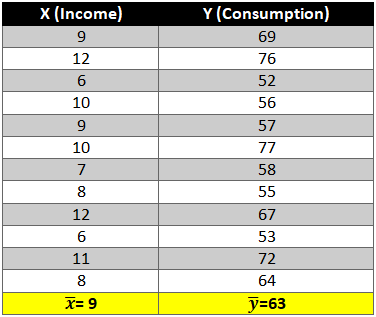
Given below is a dataset for which we will try to generate a linear function i.e.
y=b0+b1Xi
Where,
y= Dependent variable
Xi= Independent variable
b0 = Intercept (coefficient)
b1 = Slope (coefficient)
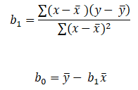
To find out beta (b0& b1) coefficients we use the following formula:-
Let’s start the calculation stepwise.
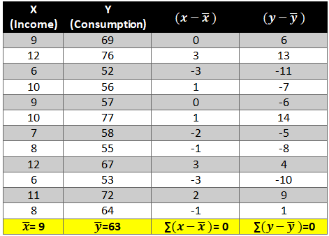
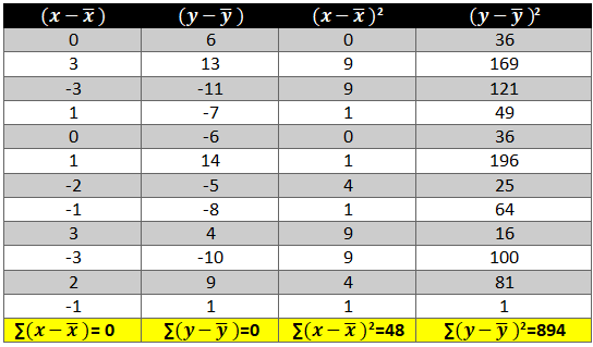
First let’s find the mean of x and y and then find out the difference between the mean values and the Xi and Yie. (x-x ̅ ) and (y-y ̅ ).
Now calculate the value of (x-x ̅ )2 and (y-y ̅ )2. The variation is squared to remove the negative signs otherwise the summation of the column will be 0.
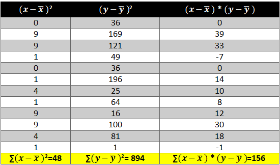
Next we need to see how income and consumption simultaneously variate i.e. (x-x ̅ )* (y-y ̅ )
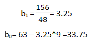
Now all there is left is to use the above calculated values in the formula:-
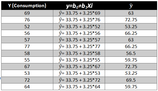
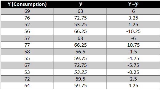
As we have the value of beta coefficients we will be able to find the y ̂(dependent variable) value.
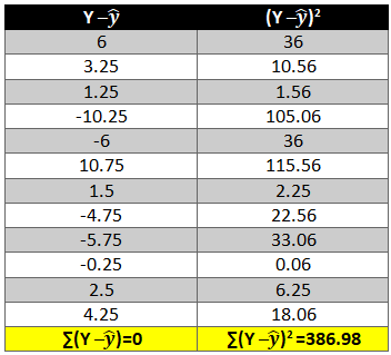
We need to now find the difference between the predicted y ̂ and observed y which is also called the error term or the error.
To remove the negative sign lets square the residual.
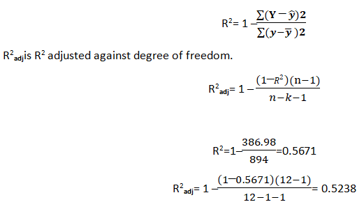
What is R2 and adjusted R2 ?
R2 also known as goodness of fit is the ratio of the difference between observed y and predicted and the observed y and the mean value of y.
Hopefully, now you have understood how to solve a Linear Regression problem and would apply what you have learned in this blog. You can also follow the video tutorial attached down the blog. You can expect more such informative posts if you keep on following the DexLab Analytics blog. DexLab Analytics provides data Science certification courses in gurgaon.
In my previous blog, I have already introduced you to a statistical term called ANOVA and I have also explained you what one-way ANOVA is? Now in this particular blog I will explain the meaning of two-way ANOVA.
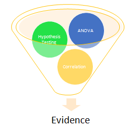
The below image shows few tests to check the relationship/variation among variables or samples. When it comes to research analysis the first thing that we should do is to understand the sample which we have and then try to disintegrate the dataset to form and understand the relationship between two or more variables to derive some kind of conclusion. Once the relation has been established, our job is to test that relationship between variables so that we have a solid evidence for or against them. In case we have to check for variation among different samples, for example if the quality of seed is affecting the productivity we have to test if it is happening by chance or because of some reason. Under these kind of situations one-way ANOVA comes in handy (analysis on the basis of a single factor).
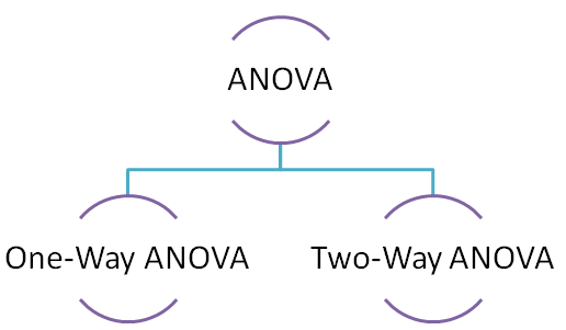
Two-way ANOVA
Two-way ANOVA is used when we are testing the variations among samples on the basis two factors. For example testing variation on the basis of seed quality and fertilizer.
Hopefully you have understood what Two-way ANOVA is. If you need more information, check out the video tutorial attached down the blog. Keep on following the DexLab Analytics blog, to find more information about Data Science, Artificial Intelligence. DexLab Analytics offers data Science certification courses in gurgaon.
Sampling is a technique in which a predefined number of observation is taken from a large population for the purpose of statistical analysis and research.
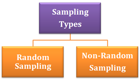
There are two types of sampling techniques:-
Random Sampling
Random sampling is a sampling technique in which each observation has an equal probability of being chosen. This kind of sample should be an unbiased representation of the population.
Types of random sampling
Simple Random Sampling:- Simple random sampling is a technique in which any observation can be chosen and each observation has an equal probability of being selected.
Stratified Random Sampling:- In this sampling technique we create sub-group of the population with similar attributes and characteristics and then out of those sub-groups we then include each category in our sample with the probability of choosing each observation from the sub-group being equal.
Systematic Sampling:- This is a sampling technique where the first observation is selected randomly and then every kth element is chosen randomly to be included in our sample. k= 2, here the first observation is selected randomly and after that every second element is included in the sample.
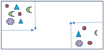
Cluster Sampling:- This is a sampling technique in which the data is grouped into small sub-groups called clusters with random categories and then from those clusters random observation is selected which then is included in the sample.
Two clusters are created from which then random observation will be chosen to form the sample.
Non-Random Sampling :- It is a sampling technique in which an element of biasedness is introduced which means that an observation is selected for the sample on the basis of not probability but choice.
Types of non-random sampling:-
Convenience Sampling:- When a sample observation is drawn from the population based on how comfortable it is for you to take the observation it is called convenience sampling. For example when you have a survey sheet that is to be filled by students from all the departments of your college but you only ask your friends to fill the survey sheet.
Judgment Sampling:– When the sample observation drawn from the population is based on your professional judgment or past experience, it is called judgment sampling.
Quota Sampling:– When you draw a sample observation from the population that is based on some specific attribute, it is called quota sampling. For example, taking sample of people over and above 50 years.
Snow Ball Sampling:– When survey subjects are selected based on referral from other survey respondents, it is called snow ball sampling.
Sampling and Non-sampling errors
Sampling errors:- It occurs when the sample is not representative of the entire population. For example a sample of 10 people with or without COVID-19 cannot tell whether or not the entire population of a country is COVID positive.
Non-sampling error:-This kind of error occurs during data collection. For example, during data collection if you falsely specified a name, it will be considered a non-sampling error.
So, with that this discussion on Sampling wraps up, hopefully, at the end of this you have learned what Sampling is, what are its variations and how do they all work. If you need further clarification, then check out our video tutorial on Sampling attached down the blog. DexLab Analytics provides the best data science course in gurgaon, keep following the blog section to stay updated.
You must be familiar with the phrase hypothesis testing, but, might not have a very clear notion regarding what hypothesis testing is all about. So, basically the term refers to testing a new theory against an old theory. But, you need to delve deeper to gain in-depth knowledge.
Hypothesis are tentative explanations of a principal operating in nature. Hypothesis testing is a statistical method which helps you prove or disapprove a pre-existing theory.
Hypothesis testing can be done to check whether the average salary of all the employees has increased or not based on the previous year’s data, testing can be done to check if the percentage of passengers increased or not in the business class due to introduction of a new service and testing can also be done to check the differences in the productivity varied land.
There are two key concepts in testing of hypothesis:-
Null Hypothesis:- It means the old theory is correct, nothing new is happening, the system is in control, old standard is correct etc. This is the theory you want to check if is true or not. For example if a ice-cream factory owner says that their ice-cream contains 90% milk, this can be written as:-
Alternative Hypothesis:- It means new theory is correct, something is happening, system is out of control, there are new standards etc. This is the theory you check against the null hypothesis. For example you say that ice-cream does not contain 90% milk, this can be written as:-
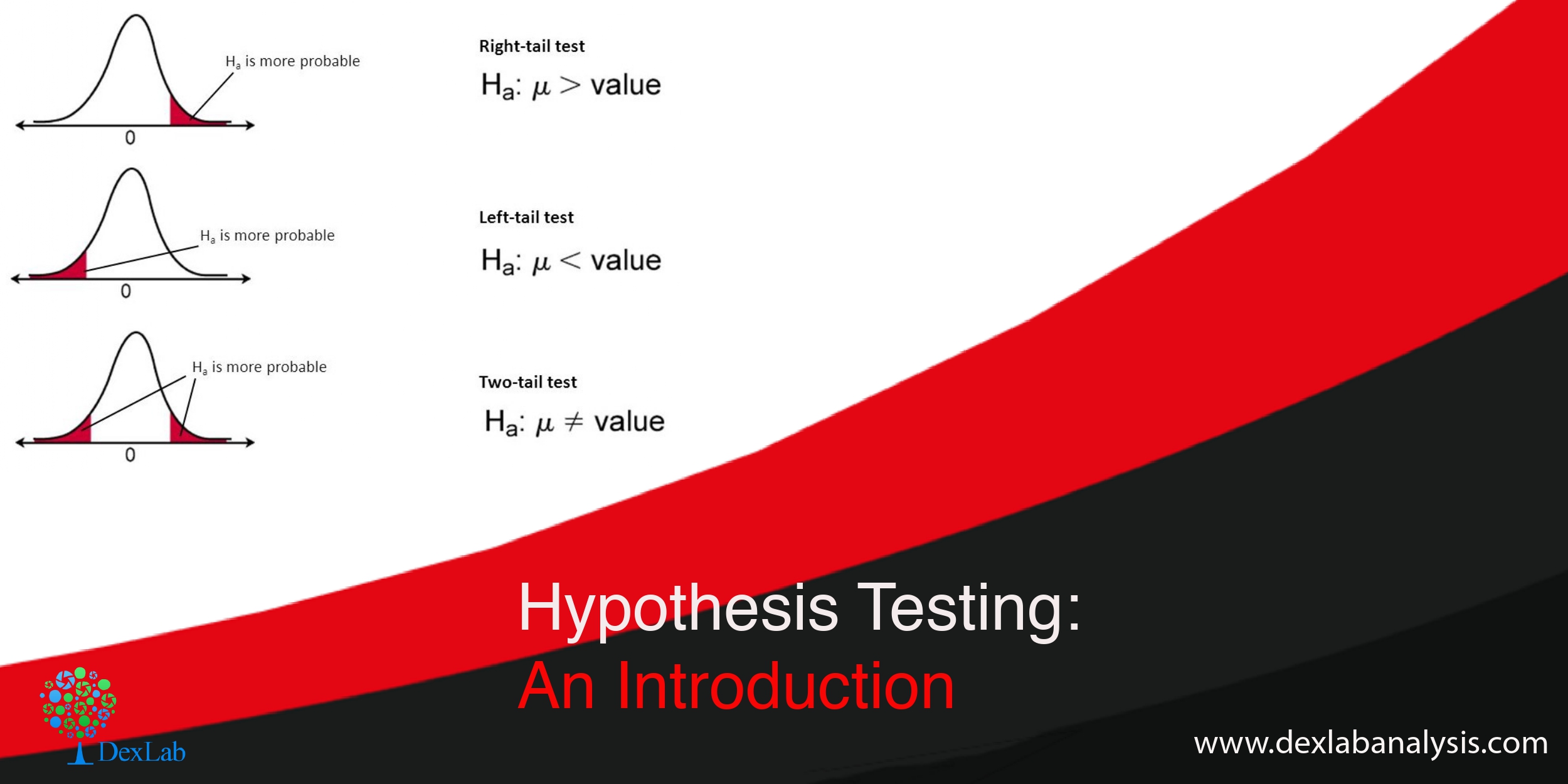
Two-tailed, right tailed and left tailed test
Two-tailed test:- When the test can take any value greater or less than 90% in the alternative it is called two-tailed test ( H190%) i.e. you do not care if the alternative is more or less all you want to know is if it is equal to 90% or no.
Right tailed test:-When your test can take any value greater than 90% (H1>90%) in the alternative hypothesis it is called right tailed test.
Left tailed test:-When your test can take any value less than 90% (H1<90%) in the alternative hypothesis it is called left tailed test.
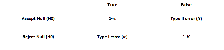
Type I error and Type II error
->When we reject the null hypothesis when it is true we are committing type I error. It is also called significance level.
->When we accept the null hypothesis when it is false we are committing type II error.
Steps involved in hypothesis testing
Build a hypothesis.
Collect data
Select significance level i.e. probability of committing type I error
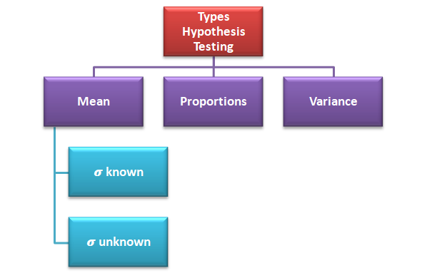
Select testing method i.e. testing of mean, proportion or variance
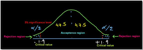
Based on the significance level find the critical value which is nothing but the value which divides the acceptance region from the rejection region
Based on the hypothesis build a two-tailed or one-tailed (right or left) test graph
Apply the statistical formula
Check if the statistical test falls in the acceptance region or the rejection region and then accept or reject the null hypothesis
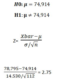
Example:- Suppose the average annual salary of the employees in a company in 2018 was 74,914. Now you want to check whether the average salary of the employees has increased or not in 2019. So, a sample of 112 people were taken and it was found out that the average annual salary of the employees in 2019 is 78,795. σ=14.530.
We will apply hypothesis testing of mean when known with 5% of significance level.
The test result shows that 2.75 falls beyond the critical value of 1.9 we reject the null hypothesis which basically means that the average salary has increased significantly in 2019 compared to 2018.
So, now that we have reached at the end of the discussion, you must have grasped the fundamentals of hypothesis testing. Check out the video attached below for more information. You can find informative posts on Data Science course, on Dexlab Analytics blog.
In this blog, we are going to be discussing a statistical technique, ANOVA, which is used for comparison.
The basic principal of ANOVA is to test for differences among the mean of different samples. It examines the amount of variation within each of these samples and the amount of variation between the samples. ANOVA is important in the context of all those situations where we want to compare more than two samples as in comparing the yield of crop from several variety of seeds etc.
The essence of ANOVA is that the total amount of variation in a set of data is broken in two types:-
The amount that can be attributed to chance.
The amount which can be attributed to specified cause.
One-way ANOVA
Under the one-way ANOVA we compare the samples based on a single factor. For example productivity of different variety of seeds.
Stepwise process involved in calculation of one-way ANOVA is as follows:-
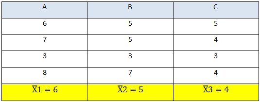
Calculate the mean of each sample X ̅
Calculate the super mean
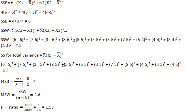
Calculate the sum of squares between (SSB) samples
Divide the result by the degree of freedom between the samples to obtain mean square between (MSW) samples.
Now calculate variation within the samples i.e. sum of square within (SSW)
Calculate mean square within (MSW)
Calculate the F-ratio
Last but not the least calculate the total variation in the given samples i.e. sum of square for total variance.
Lets now solve a one-way ANOVA problem.
A,B and C are three different variety of seeds and now we need to check if there is any variation in their productivity or not. We will be using one-way ANOVA as there is a single factor comparison involved i.e. variety of seeds.
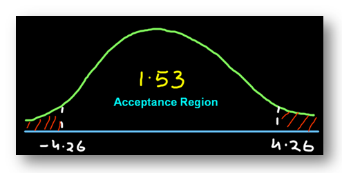
The f-ratio is 1.53 which lies within the critical value of 4.26 (calculated from the f-distribution table).
Conclusion:- Since the f-ratio lies within the acceptance region we can say that there is no difference in the productivity of the seeds and the little bit of variation that we see is caused by chance.
Two-way ANOVA will be discussed in my next blog so do comeback for the update.
Hopefully, you have found this blog informative, for more clarification watch the video attached down the blog. You can find more such posts on Data Science course topics, just keep on following the DexLab Analytics blog.
Today’s workspace has turned volatile in trying to adjust to the new normal. Along with struggling to stay indoors while living a virtual life, adopting new manners of social distancing, people are also having to deal with issues like job loss, pay cut, or, worse, lack of vacancies. Different sectors are getting hit, except for those driven by cutting edge technology like Data Science, Artificial intelligence. The need to transition into a digital world is greater than ever. As per the World Economic Forum, there would be a greater push towards “digitization” as well as “automation”. This signifies the need for professionals with a background in Data Science, Artificial Intelligence in the future that is going to be entirely data-reliant.
So, what are you going to do? Sit back and wait till the storm passes over or are you going to utilize this downtime to upskill yourself with a Data Science course? With the PM stressing on how the “skill, re-skill and upskill” being the need of the hour, you can hardly afford to lose more time. Since Data Science is one of the comparatively steadier fields, that is growing despite all odds, it is time to acquire data literacy to stay relevant in a workspace that is increasingly becoming data-driven. From healthcare to manufacturing, different sectors are busy decoding the data in hand to go digital in a pandemic ridden world, and employers are looking for people who are willing to push the envelope harder to remain relevant.
What is data literacy?
Before progressing, you must understand what data literacy even means. Data literacy basically refers to having an in-depth knowledge of data that helps the employees work with data to derive actionable information from it and channelizing that to make informed decisions. However, data literacy has a wider meaning and it is not limited to the data team comprising data scientists, no, it takes all the employees in its ambit, so, that the data flow throughout the organization is seamless. Without there being employees who know their way around data, an organization can never realize its dream of initiating a data-driven culture. Having a background in Data science using Python training is the key to achieving data literacy.
The demand for data scientists and data analysts is soaring up
Despite the ominous presence of the pandemic, the demand for Data Science professionals is there and in August, the demand for Data Analysts and Data Scientists soared. As per a recent study, in India, a Data Science professional can expect no less than ₹9.5 lakh per annum. With prestigious institutes like Infosys, IBM India, Cognizant Technology Solutions, Accenture hiring, it is now absolutely mandatory to undergo Data Science training to grab the job opportunities.
Getting Data Science certification can help you close the gap
The skill gap is there, but, that does not mean it could not be taken care of. On the contrary, it is absolutely possible and imperative that you take the necessary step of upskilling yourself to be ready for the Data Science field. Having a working knowledge of data is not enough, you must be familiar with the latest Data Science tools, must possess the knowledge to work with different models, must be familiar with data extraction, data manipulation. All of these skills and more, you would need to master before you go seeking a well-paying job.
Self-study might seem like a tempting idea, but, it is not a practical solution, if you want to be industry-ready then you must know what the industry is expecting from a Data Science professional, and only a faculty comprising industry experts can give you that knowledge while guiding you through a well designed Python for data science training course.
An institute such as DexLab Analytics understands the need of the hour and has a great team of industry professionals and experts to help aspiring Data Scientists and Data Analysts fulfill their dream. Along with offering state-of-the-art Data Science certification courses, they also provide courses like Machine Learning Using Python.
No matter which way you look, upskilling is the need of the hour as the world is busy embracing the power of Data Science. Stop procrastinating and get ready for the future.
In this blog we are discussing automation, a function for automating data preparation using a mix of Python libraries. So let’s start.
Problem statement
A data containing the following observation is given to you in which the first row contains column headers and all the other rows contains the data. Some of the rows are faulty, a row is faulty if it contains at least one cell with a NULL value. You are supposed to delete all the faulty rows containing NULL value written in it.
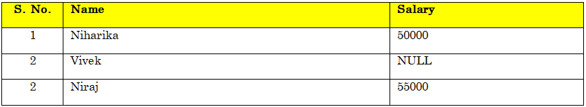
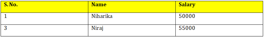
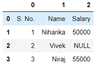
In the table given below, the second row is faulty, it contains a NULL value in salary column. The first row is never faulty as it contains the column headers. In the data provided to you every cell in a column may contain a single word and each word may contain digits between 0 & 9 or lowercase and upper case English letters. For example:
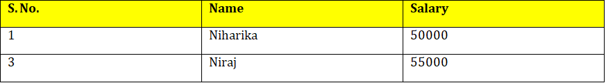
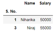
In the above example after removing the faulty row the table looks like this:
The order of rows cannot be changed but the number of rows and columns may differ in different test case.
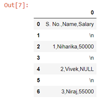
The data after preparation must be saved in a CSV format. Every two successive cells in each row are separated by a single comma ‘,’symbol and every two successive rows are separated by a new-line ‘\n’ symbol. For example, the first table from the task statement to be saved in a CSV format is a single string ‘S. No., Name, Salary\n1,Niharika,50000\n2,Vivek,NULL\n3,Niraj,55000’ . The only assumption in this task is that each row may contain same number of cells.
Write a python function that converts the above string into the given format.
Write a function:
def Solution(s)
Given a string S of length N, returns the table without the Faulty rows in a CSV format.
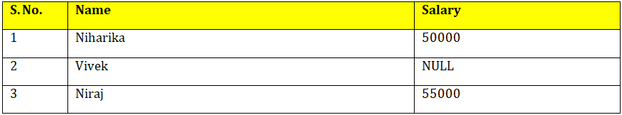
Given S=‘S. No., Name, Salary\n1,Niharika,50000\n2,Vivek,NULL\n3,Niraj,55000’
The table with data from string S looks as follows:
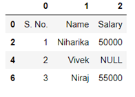
After removing the rows containing the NULL values the table should look like this:
You can try a number of strings to cross-validate the function you have created.
Let’s begin.
First we will store the string in a variable s
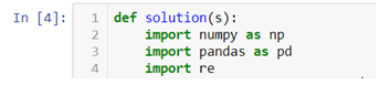
Now we will start by declaring the function name and importing all the necessary libraries.
Creating a pattern to separate the string from ‘\n’ .
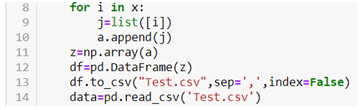
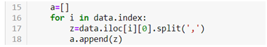
Creating a loop to create multiple lists within a list.
In the above code the list is converted to an array and then used to create a dataframe and stored as csv file in the default working directory.
Now we need to split the string to create multiple columns.
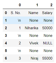
The above code creates a dataframe with multiple columns.
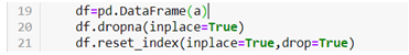
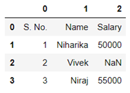
Now after dropping the rows with NaN values data looks like
To reset the index we can now use .reset_index() method.
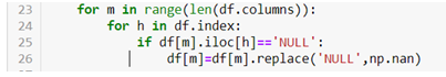
Now the problem with the above dataframe created is that the NULL values are in string format, so first we need to convert them into NaN values and then only we will be able to drop them. For that we will be using the following code.
Now we will be able to drop the NaN values easily by using .dropna() method.
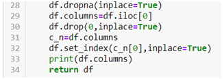
In the above code we first dropped the NaN values then we used the first row of the data set to create column names and then dropped the original row. We also made the first column as index.
Hence we have managed to create a function that can give us the above data. Once created this function can be used to convert a string into dataframe with similar pattern.
Hopefully, you found the discussion informative enough. For further clarification watch the video attached below the blog. To access more informative blogs on Data science using python training related topics, keep on following the Dexlab Analytics blog.
Here’s a video introduction to Automation. You can check it down below to develop a considerable understanding of the same:
The world has finally woken up and smelled the power of data science and now we are living in a world that is being driven by data. There is no denying the fact that new technologies are coming to the fore that are born out of data-driven insight and numerous sectors are also turning towards data science techniques and tools to increase their operational efficiency.
This in turn is also pushing a demand for skilled people in various sectors who are armed with Data Science course or, Retail Analytics Courses to be able to sift through mountains of data to clean it, sort it and analyze it for uncovering valuable information. Decisions that were earlier taken often on the basis of erroneous data or, assumption can now be more accurate thanks to application of data science.
Now let’s take a look at which sectors are benefitting the most from data science
Healthcare
The healthcare industry has adopted the data science techniques and the benefits could already be perceived. Keeping track of healthcare records is easier not just that but digging through the pile of patient data and its analysis actually helps in giving hint regarding health issues that might crop up in near future. Preventive care is now possible and also monitoring patient health is easier than ever before.
The development in the field can also predict which medication would be suitable for a particular patient. Data analytics and data science application is also enabling the professionals in this sector to offer better diagnostic results.
Retail
This is one industry that is reaping huge benefits from the application of data science. Now sorting through the customer data, survey data it is easier to gauge the customers’ mindset. Predictive analysis is helping the experts in this field to predict the personal preference of the consumers and they are able to come up with personalized recommendations that is bound to help them retain customers. Not just that they can also find the problem areas in their current marketing strategy to make changes accordingly.
Transport
Transport is another sector that is using data science techniques to its advantage and in turn it is increasing its service quality. Both the public and private transportation services providers are keeping track of customer journey and getting the details necessary to develop personalized information, they are also helping people be prepared for unexpected issues and most importantly they are helping people reach their destinations without any glitch.
Finance
If so many industries are reaping benefits, Finance is definitely to follow suit. Dealing with valuable data regarding banking transactions, credit history is essential. Based on the data insight it is possible to offer customers personalized financial advice. Also the credit risk issue could be minimized thanks to the insight derived from a particular customer’s credit history. It would allow the financial institute make an informed decision. However, credit risk analytics training would be required for personnel working in this field.
Telecom
The field of telecom is surely a busy sector that has to deal with tons of valuable data. With the application of data science now they are able to find a smart solution to process the data they gather from various call records, messages, social media platforms in order to design and deliver services that are in accordance with customers’ individualistic needs.
Harnessing the power of data science is definitely going to impact all the industries in future. The data science domain is expanding and soon there would be more miracles to observe. Data Science training can help upskill the employees reduce the skill gap that is bugging most sectors.
This is the second part of the probability series, in the first segment we discussed the basic concepts of probability. In this second part we will delve deeper into the topic and discuss the theorems of probability. Let’s find out what these theorems are.
Addition Theorem
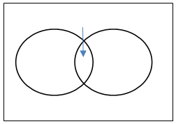
If A and B are two events and they are not necessarily mutually exclusive then the probability of occurrence of at least one of the two events A and B i.e. P(AUB) is given by
Removing the intersections will give the probability of A or B or both.
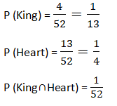
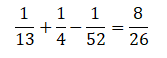
Example:- From a deck of cards 1 card is drawn, what is the probability the card is king or heart or both?
Total cards 52
P(KingUHeart)= P(King)+P(Heart) ─ P(King∩Heart)
If A and B are two mutually exclusive events then the probability that either A or B will occur is the sum of individual probabilities of the events A and B.
P(A)+P(B), here the combined probability of the two will either give P(A) or P(B)
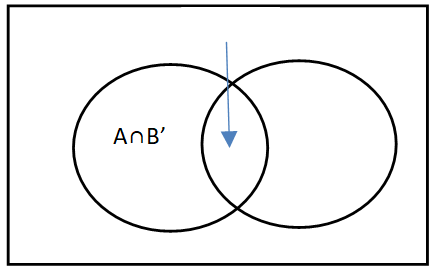
If A and B are two non mutually exclusive events then the probability of occurrence of event A is given by
Where B’ is 1-P(B), that means probability of A is calculated as P(A)=1-P(B)
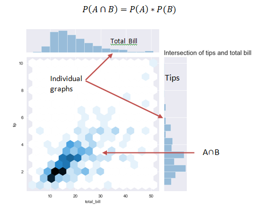
Multiplication Law
The law of multiplication is used to find the joint probability or the intersection i.e. the probability of two events occurring together at the same point of time.
In the above graph we see that when the bill is paid at the same time tip is also paid and the interaction of the two can be seen in the graph.
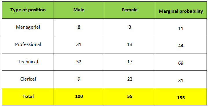
Joint probability table
A joint probability table displays the intersection (joint) probabilities along with the marginal probabilities of a given problem where the marginal probability is computed by dividing some subtotal by the whole.
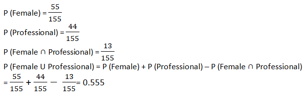
Example:- Given the following joint probability table find out the probability that the employee is female or a professional worker.
Watch this video down below that further explains the theorems.
At the end of this blog, you must have grasped the basics of the theorems discussed here. Keep on tracking the Dexlab Analytics blog where you will find more discussions on topics related to Data Science training.