Data and Risk Analytics Archives - DexLab Analytics | Big Data Hadoop SAS R Analytics Predictive Modeling & Excel VBA

MongoDB Basics Part-I

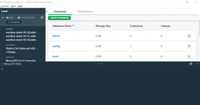
In this particular blog we will discuss about few of the basic functions of MQL (MongoDB Query Language) and we will also see how to use them? We will be using MongoDB Compass shell (MongoSH Beta) which is available in the latest version of MongoDB Compass.

Connect your Atlas cluster to your MongoDB Compass to get started. Latest version of  MongoDB Compass will have this shell, so if you don’t find this shell then please install the latest version for this to work.

Now lets start with the functions.

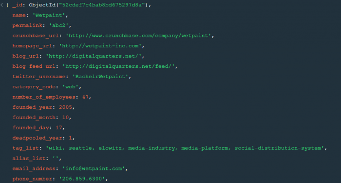
  1. find() :- You need this function for data extraction in the shell.

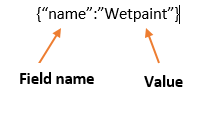
In the shell we need to first write the “use database name”  code to access the database  then use .find() to extract data which has name “Wetpaint”

For the above query we get the following result:-


The above result brings us to another function .pretty() .

2. pretty() :- this function helps us see the result more clearly.

Try it yourself to compare the results.

3. count() :- Now lets see how many entries we have by the company name “Wetpaint”.

So we have only one document.

4. Comparison operators :-

“$eq” : Equal to

“$neq”: Not equal to

“$gt”: Greater than

“$gte”: Greater than equal to

“$lt”: Less than

“$lte”: Less than equal to

Lets see how this works.

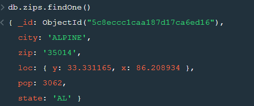
5. findOne() :- To get a single document from a collection we use this function.


6. insert() :- This is used to insert documents in a collection.

Now lets check if we have been able to insert this document or not.

Notice that a unique id has been added to the document by default. The given id has to be unique or else there will be an error. To provide a user defined  id use “_id”.


So, with that we come to the end of the discussion on the MongoDB. Hopefully it helped you understand the topic, for more information you can also watch the video tutorial attached down this blog. The blog is designed and prepared by Niharika Rai, Analytics Consultant, DexLab Analytics DexLab Analytics offers machine learning courses in Gurgaon. To keep on learning more, follow DexLab Analytics blog.


.

ARIMA (Auto-Regressive Integrated Moving Average)

arima-time series-dexlab analytics

This is another blog added to the series of time series forecasting. In this particular blog  I will be discussing about the basic concepts of ARIMA model.

So what is ARIMA?

ARIMA also known as Autoregressive Integrated Moving Average is a time series forecasting model that helps us predict the future values on the basis of the past values. This model predicts the future values on the basis of the data’s own lags and its lagged errors.

When a  data does not reflect any seasonal changes and plus it does not have a pattern of random white noise or residual then  an ARIMA model can be used for forecasting.

There are three parameters attributed to an ARIMA model p, q and d :-

p :- corresponds to the autoregressive part

q:- corresponds to the moving average part.

d:- corresponds to number of differencing required to make the data stationary.

In our previous blog we have already discussed in detail what is p and q but what we haven’t discussed is what is d and what is the meaning of differencing (a term missing in ARMA model).

Since AR is a linear regression model and works best when the independent variables are not correlated, differencing can be used to make the model stationary which is subtracting the previous value from the current value so that the prediction of any further values can be stabilized .  In case the model is already stationary the value of d=0. Therefore “differencing is the minimum number of deductions required to make the model stationary”. The order of d depends on exactly when your model becomes stationary i.e. in case  the autocorrelation is positive over 10 lags then we can do further differencing otherwise in case autocorrelation is very negative at the first lag then we have an over-differenced series.

The formula for the ARIMA model would be:-

To check if ARIMA model is suited for our dataset i.e. to check the stationary of the data we will apply Dickey Fuller test and depending on the results we will  using differencing.

In my next blog I will be discussing about how to perform time series forecasting using ARIMA model manually and what is Dickey Fuller test and how to apply that, so just keep on following us for more.

So, with that we come to the end of the discussion on the ARIMA Model. Hopefully it helped you understand the topic, for more information you can also watch the video tutorial attached down this blog. The blog is designed and prepared by Niharika Rai, Analytics Consultant, DexLab Analytics DexLab Analytics offers machine learning courses in Gurgaon. To keep on learning more, follow DexLab Analytics blog.


.

Autocorrelation- Time Series – Part 3

Autocorrelation is a special case of correlation. It refers to the relationship between successive values of the same variables .For example if an individual with a consumption pattern:-

spends too much in period 1 then he will try to compensate that in period 2 by spending less than usual. This would mean that Ut is correlated with Ut+1 . If it is plotted the graph will appear as follows :

Positive Autocorrelation : When the previous year’s error effects the current year’s error in such a way that when a graph is plotted the line moves in the upward direction or when the error of the time t-1 carries over into a positive error in the following period it is called a positive autocorrelation.
Negative Autocorrelation : When the previous year’s error effects the current year’s error in such a way that when a graph is plotted the line moves in the downward direction or when the error of the time t-1 carries over into a negative error in the following period it is called a negative autocorrelation.

Now there are two ways of detecting the presence of autocorrelation
By plotting a scatter plot of the estimated residual (ei) against one another i.e. present value of residuals are plotted against its own past value.

If most of the points fall in the 1st and the 3rd quadrants , autocorrelation will be positive since the products are positive.

If most of the points fall in the 2nd and 4th quadrant , the autocorrelation will be negative, because the products are negative.
By plotting ei against time : The successive values of ei are plotted against time would indicate the possible presence of autocorrelation .If e’s in successive time show a regular time pattern, then there is autocorrelation in the function. The autocorrelation is said to be negative if successive values of ei changes sign frequently.
First Order of Autocorrelation (AR-1)
When t-1 time period’s error affects the error of time period t (current time period), then it is called first order of autocorrelation.
AR-1 coefficient p takes values between +1 and -1
The size of this coefficient p determines the strength of autocorrelation.
A positive value of p indicates a positive autocorrelation.
A negative value of p indicates a negative autocorrelation
In case if p = 0, then this indicates there is no autocorrelation.
To explain the error term in any particular period t, we use the following formula:-

Where Vt= a random term which fulfills all the usual assumptions of OLS
How to find the value of p?

One can estimate the value of ρ by applying the following formula :-

Time Series Analysis & Modelling with Python (Part II) – Data Smoothing

dexlab_time_series

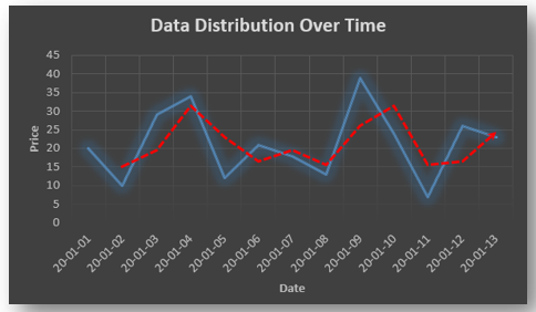
Data Smoothing is done to better understand the hidden patterns in the data. In the non- stationary processes, it is very hard to forecast the data as the variance over a period of time changes, therefore data smoothing techniques are used to smooth out the irregular roughness to see a clearer signal.

In this segment we will be discussing two of the most important data smoothing techniques :-

  • Moving average smoothing
  • Exponential smoothing

Moving average smoothing

Moving average is a technique where subsets of original data are created and then average of each subset is taken to smooth out the data and find the value in between each subset which better helps to see the trend over a period of time.

Lets take an example to better understand the problem.

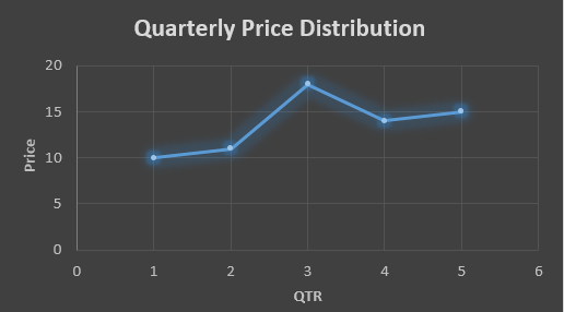
Suppose that we have a data of price observed over a period of time and it is a non-stationary data so that the tend is hard to recognize.

QTR (quarter)Price
110
211
318
414
515
6?


In the above data we don’t know the value of the 6th quarter.

….fig (1)

The plot above shows that there is no trend the data is following so to better understand the pattern we calculate the moving average over three quarter at a time so that we get in between values as well as we get the missing value of the 6th quarter.

To find the missing value of 6th quarter we will use previous three quarter’s data i.e.

MAS =  = 15.7

QTR (quarter)Price
110
211
318
414
515
615.7

MAS =  = 13

MAS =  = 14.33

QTR (quarter)PriceMAS (Price)
11010
21111
31818
41413
51514.33
615.715.7


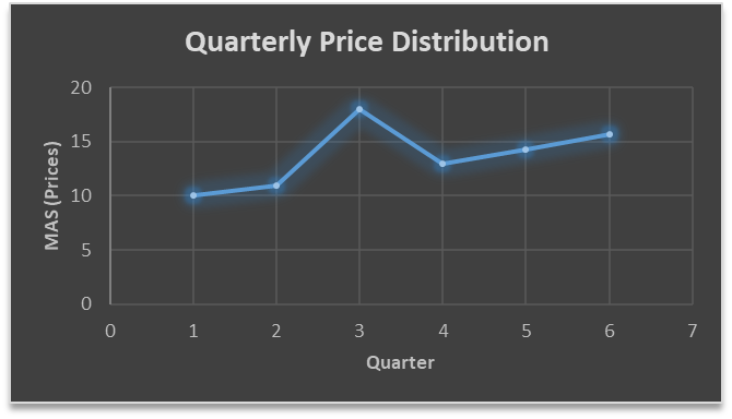
….. fig (2)

In the above graph we can see that after 3rd quarter there is an upward sloping trend in the data.

Exponential Data Smoothing

In this method a larger weight ( ) which lies between 0 & 1 is given to the most recent observations and as the observation grows more distant the weight decreases exponentially.

The weights are decided on the basis how the data is, in case the data has low movement then we will choose the value of  closer to 0 and in case the data has a lot more randomness then in that case we would like to choose the value of  closer to 1.

EMA= Ft= Ft-1 + (At-1 – Ft-1)

Now lets see a practical example.

For this example we will be taking  = 0.5

Taking the same data……

QTR (quarter)Price

(At)

EMS Price(Ft)
11010
211?
318?
414?
515?
6??


To find the value of yellow cell we need to find out the value of all the blue cells and since we do not have the initial value of F1 we will use the value of A1. Now lets do the calculation:-

F2=10+0.5(10 – 10) = 10

F3=10+0.5(11 – 10) = 10.5

F4=10.5+0.5(18 – 10.5) = 14.25

F5=14.25+0.5(14 – 14.25) = 14.13

F6=14.13+0.5(15 – 14.13)= 14.56

QTR (quarter)Price

(At)

EMS Price(Ft)
11010
21110
31810.5
41414.25
51514.13
614.5614.56

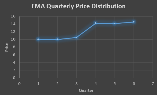
In the above graph we see that there is a trend now where the data is moving in the upward direction.

So, with that we come to the end of the discussion on the Data smoothing method. Hopefully it helped you understand the topic, for more information you can also watch the video tutorial attached down this blog. The blog is designed and prepared by Niharika Rai, Analytics Consultant, DexLab Analytics DexLab Analytics offers machine learning courses in Gurgaon. To keep on learning more, follow DexLab Analytics blog.


.

Time Series Analysis Part I


A time series is a sequence of numerical data in which each item is associated with a particular instant in time. Many sets of data appear as time series: a monthly sequence of the quantity of goods shipped from a factory, a weekly series of the number of road accidents, daily rainfall amounts, hourly observations made on the yield of a chemical process, and so on. Examples of time series abound in such fields as economics, business, engineering, the natural sciences (especially geophysics and meteorology), and the social sciences.

  • Univariate time series analysis- When we have a single sequence of data observed over time then it is called univariate time series analysis.
  • Multivariate time series analysis – When we have several sets of data for the same sequence of time periods to observe then it is called multivariate time series analysis.

The data used in time series analysis is a random variable (Yt) where t is denoted as time and such a collection of random variables ordered in time is called random or stochastic process.

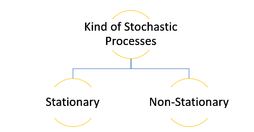
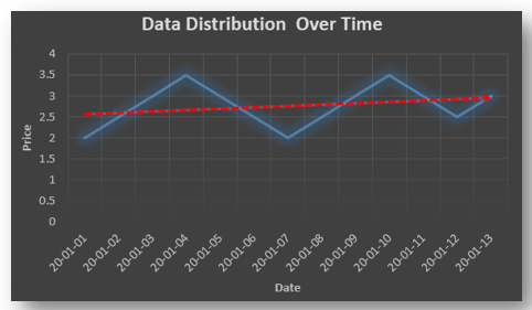
Stationary: A time series is said to be stationary when all the moments of its probability distribution i.e. mean, variance , covariance etc. are invariant over time. It becomes quite easy forecast data in this kind of situation as the hidden patterns are recognizable which make predictions easy.

Non-stationary: A non-stationary time series will have a time varying mean or time varying variance or both, which makes it impossible to generalize the time series over other time periods.

Non stationary processes can further be explained with the help of a term called Random walk models. This term or theory usually is used in stock market which assumes that stock prices are independent of each other over time. Now there are two types of random walks:
Random walk with drift : When the observation that is to be predicted at a time ‘t’ is equal to last period’s value plus a constant or a drift (α) and the residual term (ε). It can be written as
Yt= α + Yt-1 + εt
The equation shows that Yt drifts upwards or downwards depending upon α being positive or negative and the mean and the variance also increases over time.
Random walk without drift: The random walk without a drift model observes that the values to be predicted at time ‘t’ is equal to last past period’s value plus a random shock.
Yt= Yt-1 + εt
Consider that the effect in one unit shock then the process started at some time 0 with a value of Y0
When t=1
Y1= Y0 + ε1
When t=2
Y2= Y1+ ε2= Y0 + ε1+ ε2
In general,
Yt= Y0+∑ εt
In this case as t increases the variance increases indefinitely whereas the mean value of Y is equal to its initial or starting value. Therefore the random walk model without drift is a non-stationary process.

So, with that we come to the end of the discussion on the Time Series. Hopefully it helped you understand time Series, for more information you can also watch the video tutorial attached down this blog. DexLab Analytics offers machine learning courses in delhi. To keep on learning more, follow DexLab Analytics blog.


.

Bayesian Thinking & Its Underlying Principles

Bayesian Thinking & Its Underlying Principles

In the previous blog on Bayes’ Theorem, we left off at an interesting junction where we just touched upon the ideas on prior odds ratio, likelihood ratio and the resulting Posterior Odds Ratio. However, we didn’t go into much detail of what it means in real life scenarios and how should we use them.

In this blog, we will introduce the powerful concept of “Bayesian Thinking” and explain why it is so important. Bayesian Thinking is a practical application of the Bayes’ Theorem which can be used as a powerful decision-making tool too!

We’ll consider an example to understand how Bayesian Thinking is used to make sound decisions.

For the sake of simplicity, let’s imagine a management consultation firm hires only two types of employees. Let’s say, IT professionals and business consultants. You come across an employee of this firm, let’s call him Raj. You notice something about Raj instantly. Raj is shy. Now if you were asked to guess which type of employee Raj is what would be your guess?

If your guess is that Raj is an IT guy based on shyness as an attribute, then you have already fallen for one of the inherent cognitive biases. We’ll talk more about it later. But what if it can be proved Raj is actually twice as likely to be a Business Consultant?!

This is where Bayesian Thinking allows us to keep account of priors and likelihood information to predict a posterior probability.

The inherent cognitive bias you fell for is actually called – Base Rate Neglect. Base Rate Neglect occurs when we do not take into account the underlying proportion of a group in the population. Put it simply, what is the proportion of IT professionals to Business consultants in a business management firm? It would be fair to assume for every 1 IT professional, the firm hires 10 business consultants.

Another assumption could be made about shyness as an attribute. It would be fair to assume shyness is more common in IT professionals as compared to business consultants. Let’s assume, 75% of IT professionals are in fact shy corresponding to about 15% of business consultants.

Think of the proportion of employees in the firm as the prior odds. Now, think of the shyness as an attribute as the Likelihood. The figure below demonstrates when we take a product of the two, we get posterior odds.
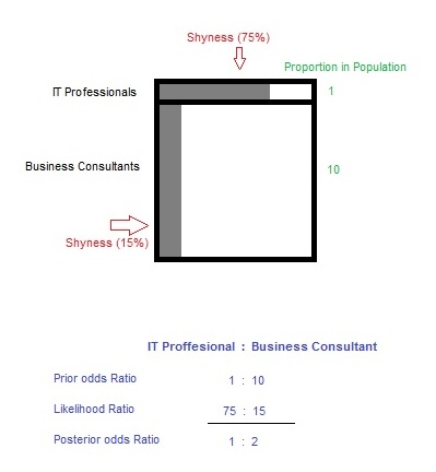
Plugging in the values shows us that Raj is actually twice as likely to be a Business consultant. This proves to us that by applying Bayesian Thinking we can eliminate bias and make a sound judgment.

Now, it would be unrealistic for you to try drawing a diagram or quantifying assumptions in most of the cases. So, how do we learn to apply Bayesian Thinking without quantifying our assumptions? Turns out we could, if we understood what are the underlying principles of Bayesian Thinking are.

Principles of Bayesian Thinking

Rule 1 – Remember your priors!

As we saw earlier how easy it is to fall for the base rate neglect trap. The underlying proportion in the population is often times neglected and we as human beings have a tendency to just focus on just the attribute. Think of priors as the underlying or the background knowledge which is essentially an additional bit of information in addition to the likelihood. A product of the priors together with likelihood determines the posterior odds/probability.

Rule 2 – Question your existing belief

This is somewhat tricky and counter-intuitive to grasp but question your priors. Present yourself with a hypothesis what if your priors were irrelevant or even wrong? How will that affect your posterior probability? Would the new posterior probability be any different than the existing one if your priors are irrelevant or even wrong?

Rule 3 – Update incrementally

We live in a dynamic world where evidence and attributes are constantly shifting. While it is okay to believe in well-tested priors and likelihoods in the present moment. However, always question does my priors & likelihood still hold true today? In other words, update your beliefs incrementally as new information or evidence surfaces. A good example of this would be the shifting sentiments of the financial markets. What holds true today, may not tomorrow? Hence, the priors and likelihoods must also be incrementally updated.

Conclusion

In conclusion, Bayesian Thinking is a powerful tool to hone your judgment skills. Developing Bayesian Thinking essentially tells us what to believe in and how much confident you are about that belief. It also allows us to shift our existing beliefs in light of new information or as the evidence unfolds. Hopefully, you now have a better understanding of Bayesian Thinking and why is it so important.

On that note, we would like to say DexLab Analytics is a premium data analytics training institute located in the heart of Delhi NCR. We provide intensive training on a plethora of data-centric subjects, including data science, Python and credit risk analytics. Stay tuned for more such interesting blogs and updates!

About the Author: Nish Lau Bakshi is a professional data scientist with an actuarial background and a passion to use the power of statistics to tackle various pressing, daily life problems.


Interested in a career in Data Analyst?

To learn more about Data Analyst with Advanced excel course – Enrol Now.
To learn more about Data Analyst with R Course – Enrol Now.
To learn more about Big Data Course – Enrol Now.

To learn more about Machine Learning Using Python and Spark – Enrol Now.
To learn more about Data Analyst with SAS Course – Enrol Now.
To learn more about Data Analyst with Apache Spark Course – Enrol Now.
To learn more about Data Analyst with Market Risk Analytics and Modelling Course – Enrol Now.
Here’s How Technology Made Education More Enjoyable and Interactive

Here’s How Technology Made Education More Enjoyable and Interactive

Technology is revamping education. The entire education system has undergone a massive change, thanks to technological advancement. The institutions are setting new goals and achieving their targets more effectively with the help of new tools and practices. These cutting edge methods not only enhances the learning approach, but also results in better interaction and fuller participation between teachers and students.

The tools of technology have turned students into active learners; they are now more engaged with their subjects. In fact, they even discover solutions to the problems on their own. The traditional lectures are now mixed with engaging illustrations and demonstrations, and classrooms are replaced with interactive sessions in which students and teachers both participate equally.

Let’s take a look at how technology has changed the classroom learning experience:

Online Classes

No longer, students have to sit through a classroom all day. If a student is interested in a particular course or subject, he or she can easily pursue degrees online without going anywhere. The internet has made interactions between students and teachers extremely easy. From the comfort of the home, anyone can learn anything.

DexLab Analytics offers Data Science Courses in Noida. Their online and classroom training is over the top.

Free educational resources found online

The internet is full of information. From a vast array of blogs, website content and applications, students as well as teachers can learn anything they desire to. Online study materials coupled with classroom learning help the students in strengthening their base on any subject as they get to learn concepts from different sources with examples and practice enough problems. This explains why students are so crazy for the internet!

2

Webinars and video streaming

The facilitators and educationists are nowadays looking up to video streaming to communicate ideas and knowledge to the students. Videos are anytime more helpful than other digital communications; they help deliver the needful content, boosting the learning abilities among the learners, while making them understand the subject matter to the core. Webinars (seminars over the web) replaces classroom seminars; teachers look up to new methods of video conferencing for smoother interaction with the students.

Podcasts

Podcasts are digital audio files. Users can easily download them. They are available over the internet for a bare subscription fee. It’s no big deal to create podcasts. Teachers can easily create podcasts that syncs well with students’ demand, thus paving a way for them to learn more efficiently. In short, podcasts allow students a certain flexibility to learn from anywhere, anytime.

Laptops, smartphones and tablets

For a better learning experience overall, both students and teachers are looking forward to better software and technology facilities. A wide number of web and mobile applications are now available for students to explore the wide horizon of education. The conventional paper notes are now replaced with e-notes that are uploaded on the internet and can be accessible from anywhere. Laptops and tablets are also used to manage course materials, research, schedules and presentations.

No second thoughts, by integrating technology with classroom training, students and teachers have an entire world to themselves. Sans the geographical limitations, they can now explore the bounties of new learning methods that are more fun and highly interactive.

DexLab Analytics appreciates the power of technology, and in accordance, have curated state of the art Data Science Courses that can be accessed both online and offline for students’ benefit. Check out the courses NOW!


The article has been sourced from – http://www.iamwire.com/2017/08/technology-teaching-education/156418


Interested in a career in Data Analyst?

To learn more about Data Analyst with Advanced excel course – Enrol Now.
To learn more about Data Analyst with R Course – Enrol Now.
To learn more about Big Data Course – Enrol Now.

To learn more about Machine Learning Using Python and Spark – Enrol Now.
To learn more about Data Analyst with SAS Course – Enrol Now.
To learn more about Data Analyst with Apache Spark Course – Enrol Now.
To learn more about Data Analyst with Market Risk Analytics and Modelling Course – Enrol Now.
Evolving Logistics Scenario: The Tech-driven Future of Logistics Industry

Customer expectations are growing by the day; they are demanding faster and more flexible deliveries at minimum delivery costs. Businesses are being pressurized to customize their manufacturing processes as per customer demands. This is a hard slog for the logistics industry, which has to keep delivering better services but for lower prices.

The logistics industry can only achieve this through ‘digital fitness’. It has to make intelligent use of the global wave of digitization, including data analytics, automation and ‘Physical Internet’. The Physical Internet is an open global logistics system that is transforming the way physical objects are handled, moved, stored and supplied. It aims towards the replacement of current logistical models and making global logistics more efficient and sustainable. The Physical Internet promises better standardization in logistics operations, including shipment sizes, labeling and systems.

The central theme in logistics sector is collaborative working, which enables market leaders to retain dominance.

Now, let us take a look at a few tech-driven domains that will shape the future of logistics.


The future of Logistics Lies in IoT

Internet of Things has been the most innovative technology of the present era. It has the potential to revolutionize the logistics sector. The key benefits of IoT with regard to logistics are:

  • Real-time alerts and notifications
  • Automate processes that gather data from various machines
  • Automate vital operations like inventory management and asset tracking: With the help of IoT, companies can improve tasks like tracking orders, determining what items need to be stocked up and how certain products are performing.
  • Able to function without any human interventions.
  • Logistic companies can provide safer deliveries
  • Enable the regulation of temperature and other environmental factors.

IoT will be advantageous for the entire logistics sector, including fleet and warehouse management, and shipment and delivery of products. IoT can help companies dealing with cargo shipments by improving visibility in the delivery and tracking of cargo.

Warehouse Automation

Warehouse automation is set for a major overhaul. Online shopping is thriving and logistics, especially warehouse operations, need to be more refined and speedy. Warehouse operations of many e-commerce giants are undergoing a robotics makeover. According to reports, the market for logistics robotics, which had generated revenues worth 1.9 billion USD in 2016, is likely to generate sky-high revenues worth 22.4 billion USD this year.

The advancements in robotics include programming robots to pick and pack goods, load and unload cargo and at times deliver goods too. Employing robots speed up the processes of data collection, maintaining records and managing inventories.  Most importantly, robots leave no room for human errors in the processes.


Blockchain Technology in Logistics

The growth of crypto-currencies like Bitcoin has popularized blockchain technology. Blockchain being a type of distributed ledger technology provides secure, traceable and transparent transactions. Blockchain technology employed by logistics firms will improve customer visibility into shipments and help prevent data breaches.

In the present times, logistics is considered the backbone of a stable economy. Thus, for India to emerge as a superpower, the logistics market needs to be developed and integrated with state-of-the-art technologies. Conducive policies and a healthy partnership between private and public sector is crucial to steer India into an era of competent and cost-effective business operations.

In times to come, automation will transform every industry. Don’t be left behind. Get an edge by enrolling for the data science and machine learning certification course at the premier data analyst training institute in DelhiDexlab Analytics.


Interested in a career in Data Analyst?

To learn more about Data Analyst with Advanced excel course – Enrol Now.
To learn more about Data Analyst with R Course – Enrol Now.
To learn more about Big Data Course – Enrol Now.

To learn more about Machine Learning Using Python and Spark – Enrol Now.
To learn more about Data Analyst with SAS Course – Enrol Now.
To learn more about Data Analyst with Apache Spark Course – Enrol Now.
To learn more about Data Analyst with Market Risk Analytics and Modelling Course – Enrol Now.
How Data Scientists are Merging Professional and Personal Resolutions for a Career Boost in 2018

The beginning of a year comes with a wide stream of promises! Some decide to work on their physique, while others look forward to visit a new country, but budding data scientists are found thinking of something else.

How Data Scientists are Merging Professional and Personal Resolutions for a Career Boost in 2018

Here goes a chart down of what goes on in a mind of a data scientist, who could stare for hours at the computer screen pondering which code or query to run…

Continue reading “How Data Scientists are Merging Professional and Personal Resolutions for a Career Boost in 2018”

Call us to know more