corporate training session Archives - DexLab Analytics | Big Data Hadoop SAS R Analytics Predictive Modeling & Excel VBA

Time Series Analysis & Modelling with Python (Part II) – Data Smoothing

Posted on January 20, 2021January 20, 2021 by Dexlab

Data Smoothing is done to better understand the hidden patterns in the data. In the non- stationary processes, it is very hard to forecast the data as the variance over a period of time changes, therefore data smoothing techniques are used to smooth out the irregular roughness to see a clearer signal.

In this segment we will be discussing two of the most important data smoothing techniques :-

Moving average smoothing
Exponential smoothing

Moving average smoothing

Moving average is a technique where subsets of original data are created and then average of each subset is taken to smooth out the data and find the value in between each subset which better helps to see the trend over a period of time.

Lets take an example to better understand the problem.

Suppose that we have a data of price observed over a period of time and it is a non-stationary data so that the tend is hard to recognize.

QTR (quarter)	Price
1	10
2	11
3	18
4	14
5	15
6	?

In the above data we don’t know the value of the 6^th quarter.

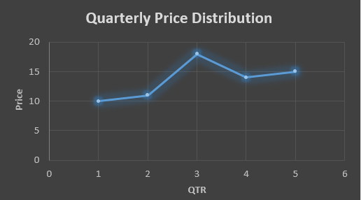
….fig (1)

The plot above shows that there is no trend the data is following so to better understand the pattern we calculate the moving average over three quarter at a time so that we get in between values as well as we get the missing value of the 6^th quarter.

To find the missing value of 6^th quarter we will use previous three quarter’s data i.e.

MAS = = 15.7

QTR (quarter)	Price
1	10
2	11
3	18
4	14
5	15
6	15.7

MAS = = 13

MAS = = 14.33

QTR (quarter)	Price	MAS (Price)
1	10	10
2	11	11
3	18	18
4	14	13
5	15	14.33
6	15.7	15.7

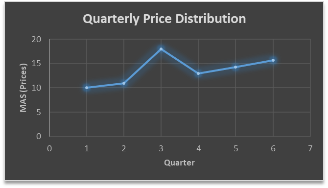
….. fig (2)

In the above graph we can see that after 3^rd quarter there is an upward sloping trend in the data.

Exponential Data Smoothing

In this method a larger weight ( ) which lies between 0 & 1 is given to the most recent observations and as the observation grows more distant the weight decreases exponentially.

The weights are decided on the basis how the data is, in case the data has low movement then we will choose the value of closer to 0 and in case the data has a lot more randomness then in that case we would like to choose the value of closer to 1.

EMA= F_t= F_t-1 + (A_t-1 – F_t-1)

Now lets see a practical example.

For this example we will be taking = 0.5

Taking the same data……

QTR (quarter)	Price (A_t)	EMS Price(F_t)
1	10	10
2	11	?
3	18	?
4	14	?
5	15	?
6	?	?

To find the value of yellow cell we need to find out the value of all the blue cells and since we do not have the initial value of F₁ we will use the value of A_1.Now lets do the calculation:-

F₂=10+0.5(10 – 10) = 10

F₃=10+0.5(11 – 10) = 10.5

F₄=10.5+0.5(18 – 10.5) = 14.25

F₅=14.25+0.5(14 – 14.25) = 14.13

F₆=14.13+0.5(15 – 14.13)= 14.56

QTR (quarter)	Price (A_t)	EMS Price(F_t)
1	10	10
2	11	10
3	18	10.5
4	14	14.25
5	15	14.13
6	14.56	14.56

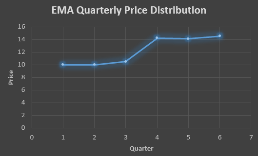
In the above graph we see that there is a trend now where the data is moving in the upward direction.

So, with that we come to the end of the discussion on the Data smoothing method. Hopefully it helped you understand the topic, for more information you can also watch the video tutorial attached down this blog. The blog is designed and prepared by Niharika Rai, Analytics Consultant, DexLab Analytics DexLab Analytics offers machine learning courses in Gurgaon. To keep on learning more, follow DexLab Analytics blog.

Time Series Analysis Part I

Posted on January 18, 2021January 18, 2021 by Dexlab

A time series is a sequence of numerical data in which each item is associated with a particular instant in time. Many sets of data appear as time series: a monthly sequence of the quantity of goods shipped from a factory, a weekly series of the number of road accidents, daily rainfall amounts, hourly observations made on the yield of a chemical process, and so on. Examples of time series abound in such fields as economics, business, engineering, the natural sciences (especially geophysics and meteorology), and the social sciences.

Univariate time series analysis- When we have a single sequence of data observed over time then it is called univariate time series analysis.
Multivariate time series analysis – When we have several sets of data for the same sequence of time periods to observe then it is called multivariate time series analysis.

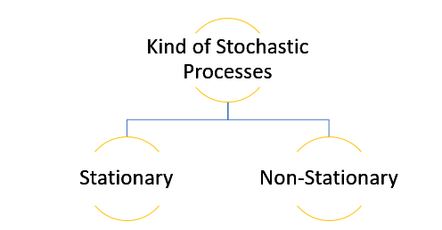
The data used in time series analysis is a random variable (Yt) where t is denoted as time and such a collection of random variables ordered in time is called random or stochastic process.

Stationary: A time series is said to be stationary when all the moments of its probability distribution i.e. mean, variance , covariance etc. are invariant over time. It becomes quite easy forecast data in this kind of situation as the hidden patterns are recognizable which make predictions easy.

Non-stationary: A non-stationary time series will have a time varying mean or time varying variance or both, which makes it impossible to generalize the time series over other time periods.

Non stationary processes can further be explained with the help of a term called Random walk models. This term or theory usually is used in stock market which assumes that stock prices are independent of each other over time. Now there are two types of random walks:
Random walk with drift : When the observation that is to be predicted at a time ‘t’ is equal to last period’s value plus a constant or a drift (α) and the residual term (ε). It can be written as
Yt= α + Yt-1 + εt
The equation shows that Yt drifts upwards or downwards depending upon α being positive or negative and the mean and the variance also increases over time.
Random walk without drift: The random walk without a drift model observes that the values to be predicted at time ‘t’ is equal to last past period’s value plus a random shock.
Yt= Yt-1 + εt
Consider that the effect in one unit shock then the process started at some time 0 with a value of Y0
When t=1
Y1= Y0 + ε1
When t=2
Y2= Y1+ ε2= Y0 + ε1+ ε2
In general,
Yt= Y0+∑ εt
In this case as t increases the variance increases indefinitely whereas the mean value of Y is equal to its initial or starting value. Therefore the random walk model without drift is a non-stationary process.

So, with that we come to the end of the discussion on the Time Series. Hopefully it helped you understand time Series, for more information you can also watch the video tutorial attached down this blog. DexLab Analytics offers machine learning courses in delhi. To keep on learning more, follow DexLab Analytics blog.

We are Proud to Host Corporate Training for WHO Reps!

Posted on February 16, 2017February 16, 2017 by Dexlab

We are happy to announce our month-long corporate training session for the representatives of WHO, who will be joining us to discuss data analytics all the way from Bhutan. The team of delegates who have come to seek training from our expert in-house trainers are for the Central of Disease Control, Ministry of Health Royal Government of Bhutan.

The training is on the concepts of R Programming, Data Science using R and Statistical Modelling using R, and will go on from the 8^th of February 2017 to the 8^th of March 2017. We are hosting this training session at our headquarters in Gurgaon, Delhi NCR. It is a matter of great pride and honour for the team of seasoned industry expert trainers at DexLab Analytics to be hosting the representatives from WHO.

Continue reading “We are Proud to Host Corporate Training for WHO Reps!”

Call us to know more

Gurgaon

Kolkata