A time series is a sequence of numerical data in which each item is associated with a particular instant in time. Many sets of data appear as time series: a monthly sequence of the quantity of goods shipped from a factory, a weekly series of the number of road accidents, daily rainfall amounts, hourly observations made on the yield of a chemical process, and so on. Examples of time series abound in such fields as economics, business, engineering, the natural sciences (especially geophysics and meteorology), and the social sciences.
Univariate time series analysis- When we have a single sequence of data observed over time then it is called univariate time series analysis.
Multivariate time series analysis – When we have several sets of data for the same sequence of time periods to observe then it is called multivariate time series analysis.
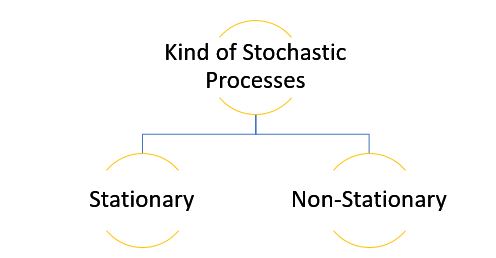
The data used in time series analysis is a random variable (Yt) where t is denoted as time and such a collection of random variables ordered in time is called random or stochastic process.
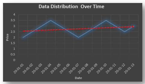
Stationary: A time series is said to be stationary when all the moments of its probability distribution i.e. mean, variance , covariance etc. are invariant over time. It becomes quite easy forecast data in this kind of situation as the hidden patterns are recognizable which make predictions easy.
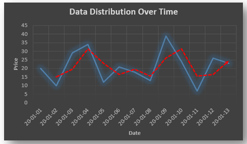
Non-stationary: A non-stationary time series will have a time varying mean or time varying variance or both, which makes it impossible to generalize the time series over other time periods.
Non stationary processes can further be explained with the help of a term called Random walk models. This term or theory usually is used in stock market which assumes that stock prices are independent of each other over time. Now there are two types of random walks: Random walk with drift : When the observation that is to be predicted at a time ‘t’ is equal to last period’s value plus a constant or a drift (α) and the residual term (ε). It can be written as Yt= α + Yt-1 + εt The equation shows that Yt drifts upwards or downwards depending upon α being positive or negative and the mean and the variance also increases over time. Random walk without drift: The random walk without a drift model observes that the values to be predicted at time ‘t’ is equal to last past period’s value plus a random shock. Yt= Yt-1 + εt Consider that the effect in one unit shock then the process started at some time 0 with a value of Y0 When t=1 Y1= Y0 + ε1 When t=2 Y2= Y1+ ε2= Y0 + ε1+ ε2 In general, Yt= Y0+∑ εt In this case as t increases the variance increases indefinitely whereas the mean value of Y is equal to its initial or starting value. Therefore the random walk model without drift is a non-stationary process.
So, with that we come to the end of the discussion on the Time Series. Hopefully it helped you understand time Series, for more information you can also watch the video tutorial attached down this blog. DexLab Analytics offers machine learning courses in delhi. To keep on learning more, follow DexLab Analytics blog.
In this fifth part of the basic of statistical inference series you will learn about different types of Parametric tests. Parametric statistical test basically is concerned with making assumption regarding the population parameters and the distributions the data comes from. In this particular segment the discussion would focus on explaining different kinds of parametric tests. You can find the 4th part of the series here.
INTRODUCTION
Parametric statistics are the most common type of inferential statistics. Inferential statistics are calculated with the purpose of generalizing the findings of a sample to the population it represents, and they can be classified as either parametric or non-parametric. Parametric tests make assumptions about the parameters of a population, whereas nonparametric tests do not include such assumptions or include fewer. For instance, parametric tests assume that the sample has been randomly selected from the population it represents and that the distribution of data in the population has a known underlying distribution. The most common distribution assumption is that the distribution is normal. Other distributions include the binomial distribution (logistic regression) and the Poisson distribution (Poisson regression).
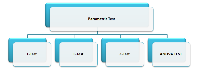
PARAMETRIC TEST
A parameter in statistics refers to an aspect of a population, as opposed to a statistic, which refers to an aspect, about a sample. For example, the population mean is a parameter, while the sample mean is a statistic. A parametric statistical test makes an assumption about the population parameters and the distributions that the data comes from. These types of tests assume to data is from normal distribution.
Data that is assumed to have been drawn from a particular distribution, and that is used in a parametric test.
Parametric equations are used in calculus to deal with the problems that arise when trying to find functions that describe curves. These equations are beyond the scope of this site, but you can find an excellent rundown of how to use these types of equations here.
The parametric tests are: Let’s discuss about each test in details.
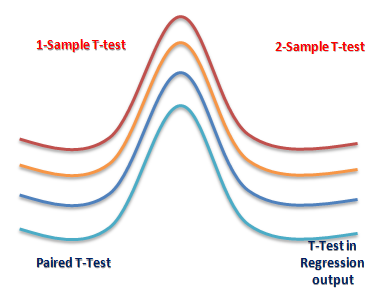
T-TEST
The T-test is one of, inferential statistics. It is used to determine whether there is a significant difference between the means of two groups or not. When the difference between two population averages is being investigated, a t-test is used. In other words, a t-test is used when we wish to compare two means. Essentially, a t-test allows us to compare the average values of the two data sets and determine if they came from the same population. In the above examples, if we were to take a sample of students from class A and another sample of students from class B, we would not expect them to have exactly the same mean and standard deviation.
Mathematically, the t-test takes a sample from each of the two sets and establishes the problem statement by assuming a null hypothesis that the two means are equal. Based on the applicable formulas, certain values are calculated and compared against the standard values, and the assumed null hypothesis is accepted or rejected accordingly.
If the null hypothesis qualifies to be rejected, it indicates that data readings are strong and are probably not due to chance. The t-test is just one of many tests used for this purpose. Statisticians must additionally use tests other than the t-test to examine more variables and tests with larger sample sizes. For a large sample size, statisticians use a z-test. Other testing options include the chi-square test and the f-test.
T-Test Assumptions
The first assumption made regarding t-tests concerns the scale of measurement. The assumption for a t-test is that the scale of measurement applied to the data collected follows a continuous or ordinal scale, such as the scores for an IQ test.
The second assumption made is that of a simple random sample, that the data is collected from a representative, randomly selected portion of the total population.
The third assumption is the data, when plotted, results in a normal distribution, bell-shaped distribution curve.
The final assumption is the homogeneity of variance. Homogeneous, or equal, variance exists when the standard deviations of samples are approximately equal.
There are three types to T-test: (i) Correlated or paired T-test, (ii) Equal variance(or pooled) T-test (iii) Unequal variance T-test.
Z-TEST
A z-test is a statistical test used to determine whether two population means are different when the variances are known and the sample size is large. The test statistic is assumed to have a normal distribution, and nuisance parameters such as standard deviation should be known in order for an accurate z-test to be performed. A z-statistic, or z-score, is a number representing how many standard deviations above or below the mean population a score derived from a z-test is.
The z-test is also a hypothesis test in which the z-statistic follows a normal distribution. The z-test is best used for greater-than-30 samples because, under the central limit theorem, as the number of samples gets larger, the samples are considered to be approximately normally distributed. When conducting a z-test, the null and alternative hypotheses, alpha and z-score should be stated. Next, the test statistic should be calculated, and the results and conclusion stated. Examples of tests that can be conducted as z-tests include a one-sample location test, a two-sample location test, a paired difference test, and a maximum likelihood estimate. Z-tests are closely related to t-tests, but t-tests are best performed when an experiment has a small sample size. Also, t-tests assume the standard deviation is unknown, while z-tests assume it is known. If the standard deviation of the population is unknown, the assumption of the sample variance equaling the population variance is made.
One Sample Z-test: A one sample z test is one of the most basic types of hypothesis test. In order to run a one sample z test, its work through several steps:
Step 1: Null hypothesis is one of the common stumbling blocks–in order to make sense of your sample and have the one sample z test give you the right information it must make sure written the null hypothesis and alternate hypothesis correctly. For example, you might be asked to test the hypothesis that the mean weight gain of an women was more than 30 pounds. Your null hypothesis would be: H0 : μ = 30 and your alternate hypothesis would be H, sub>1: μ > 30.
Step 2: Use the z-formula to find a z-score
All you do is put in the values you are given into the formula. Your question should give you the sample mean (x̄), the standard deviation (σ), and the number of items in the sample (n). Your hypothesized mean (in other words, the mean you are testing the hypothesis for, or your null hypothesis) is μ0 .
Two Sample Z Test: The z-Test: Two- Sample for Means tool runs a two sample z-Test means with known variances to test the null hypothesis that there is no difference between the means of two independent populations. This tool can be used to run a one-sided or two-sided test z-test.
ANOVA
Analysis of variance (ANOVA) is an analysis tool used in statistics that splits an observed aggregate variability found inside a data set into two parts: systematic factors and random factors. The systematic factors have a statistical influence on the given data set, while the random factors do not. Analysts use the ANOVA test to determine the influence that independent variables have on the dependent variable in a regression study. The ANOVA test is the initial step in analysing factors that affect a given data set. Once the test is finished, an analyst performs additional testing on the methodical factors that measurably contribute to the data set’s inconsistency. The analyst utilizes the ANOVA test results in an f-test to generate additional data that aligns with the proposed regression models. The ANOVA test allows a comparison of more than two groups at the same time to determine whether a relationship exists between them. The result of the ANOVA formula, the F statistic (also called the F-ratio), allows for the analysis of multiple groups of data to determine the variability between samples and within samples.
If no real difference exists between the tested groups, which is called the null hypothesis, the result of the ANOVA’s F-ratio statistic will be close to 1. Fluctuations in its sampling will likely follow the Fisher F distribution. This is actually a group of distribution functions, with two characteristic numbers, called the numerator degrees of freedom and the denominator degrees of freedom.
One-way Anova: A one-way ANOVA uses one independent variable, use a one-way ANOVA when collected data about one categorical independent variable and one quantitative dependent variable. The independent variable should have at least three levels (i.e. at least three different groups or categories). ANOVA that if the dependent variable changes according to the level of the independent variable.
Two-way Anova: A two-way ANOVA is used to estimate how the mean of a quantitative variable changes according to the levels of two categorical variables. Use a two-way ANOVA when you want to know how two independent variables, in combination, affect a dependent variable.
F-TEST
An “F Test” is a catch-all term for any test that uses the F-distribution. In most cases, when people talk about the F-Test, what they are actually talking about is The F-Test to compare two variances. However, the f-statistic is used in a variety of tests including regression analysis, the Chow test and the Scheffe Test (a post-hoc ANOVA test).
F Test to Compare Two Variances
A Statistical F Test uses an F Statistic to compare two variances, s1 and s2 , by dividing them. The result is always a positive number (because variances are always positive). The equation for comparing two variances with the f-test is:
If the variances are equal, the ratio of the variances will equal 1. For example, if you had two data sets with a sample 1 (variance of 10) and a sample 2 (variance of 10), the ratio would be 10/10 = 1.
You always test that the population variances are equal when running an F Test. In other words, you always assume that the variances are equal to 1. Therefore, your null hypothesis will always be that the variances are equal. Assumptions
Several assumptions are made for the test. Your population must be approximately normally distributed (i.e. fit the shape of a bell curve) in order to use the test. Plus, the samples must be independent events. In addition, you’ll want to bear in mind a few important points:
The larger variance should always go in the numerator (the top number) to force the test into a right-tailed test. Right-tailed tests are easier to calculate.
For two-tailed tests, divide alpha by 2 before finding the right critical value.
If you are given standard deviations, they must be squared to get the variances.
If your degrees of freedom aren’t listed in the F Table, use the larger critical value. This helps to avoid the possibility of Type I errors.
CONCLUSION
Conventional statistical procedures may also call parametric tests. In every parametric test, for example, you have to use statistics to estimate the parameter of the population. Because of such estimation, you have to follow a process that includes a sample as well as a sampling distribution and a population along with certain parametric assumptions that required, which makes sure that all components compatible with one another.
An example can use to explain this. Observations are first of all quite independent, the sample data doesn’t have any normal distributions and the scores in the different groups have some homogeneous variances. Parametric tests are based on the distribution, parametric statistical tests are only applicable to the variables. There’re no parametric tests that exist for the nominal scale date, and finally, they are quite powerful when they exist. There are mainly four types of Parametric Hypothesis Test which already mentioned in previous slides.
Advantages of Parametric Test
One of the biggest and best advantages of using parametric tests is first of all that you don’t need much data that could be converted in some order or format of ranks. The process of conversion is something that appears in rank format and to be able to use a parametric test regularly, you will end up with a severe loss in precision. Another big advantage of using parametric tests is the fact that you can calculate everything so easily. In short, you will be able to find software much quicker so that you can calculate them fast and quick. Apart from parametric tests, there are other non-parametric tests, where the distributors are quite different and they are not all that easy when it comes to testing such questions that focus related to the means and shapes of such distributions.
Disadvantages of Parametric Test
Parametric tests are not valid when it comes to small data sets. The requirement that the populations are not still valid on the small sets of data, the requirement that the populations which are under study have the same kind of variance and the need for such variables are being tested and have been measured at the same scale of intervals. Another disadvantage of parametric tests is that the size of the sample is always very big, something you will not find among non-parametric tests. That makes it a little difficult to carry out the whole test.
This particular discussion on parametric tests ends here, and at the end of this you must have developed clear ideas regarding these test categories. To find more such posts on Data Science training topics follow the Dexlab Analytics blog.
In this series we cover the basic of statistical inference, this is the fourth part of our discussion where we explain the concept of hypothesis testing which is a statistical technique. You could also check out the 3rd part of the series here.
Introduction
The objective of sampling is to study the features of the population on the basis of sample observations. A carefully selected sample is expected to reveal these features, and hence we shall infer about the population from a statistical analysis of the sample. This process is known as Statistical Inference.
There are two types of problems. Firstly, we may have no information at all about some characteristics of the population, especially the values of the parameters involved in the distribution, and it is required to obtain estimates of these parameters. This is the problem of Estimation. Secondly, some information or hypothetical values of the parameters may be available, and it is required to test how far the hypothesis is tenable in the light of the information provided by the sample. This is the problem of Test of Hypothesis or Test of Significance.
In many practical problems, statisticians are called upon to make decisions about a population on the basis of sample observations. For example, given a random sample, it may be required to decide whether the population, from which the sample has been obtained, is a normal distribution with mean = 40 and s.d. = 3 or not. In attempting to reach such decisions, it is necessary to make certain assumptions or guesses about the characteristics of population, particularly about the probability distribution or the values of its parameters. Such an assumption or statement about the population is called Statistical Hypothesis. The validity of a hypothesis will be tested by analyzing the sample. The procedure which enables us to decide whether a certain hypothesis is true or not, is called Test of Significance or Test of Hypothesis.
What Is Testing Of Hypothesis?
Statistical Hypothesis
Hypothesis is a statistical statement or a conjecture about the value of a parameter. The basic hypothesis being tested is called the null hypothesis. It is sometimes regarded as representing the current state of knowledge & belief about the value being tested. In a test the null hypothesis is constructed with alternative hypothesis denoted by 𝐻1 ,when a hypothesis is completely specified then it is called a simple hypothesis, when all factors of a distribution are not known then the hypothesis is known as a composite hypothesis.
Testing Of Hypothesis
The entire process of statistical inference is mainly inductive in nature, i.e., it is based on deciding the characteristics of the population on the basis of sample study. Such a decision always involves an element of risk i.e., the risk of taking wrong decisions. It is here that modern theory of probability plays a vital role & the statistical technique that helps us at arriving at the criterion for such decision is known as the testing of hypothesis.
Testing Of Statistical Hypothesis
A test of a statistical hypothesis is a two action decision after observing a random sample from the given population. The two action being the acceptance or rejection of hypothesis under consideration. Therefore a test is a rule which divides the entire sample space into two subsets.
A region is which the data is consistent with 𝐻0.
The second is its complement in which the data is inconsistent with 𝐻0.
The actual decision is however based on the values of the suitable functions of the data, the test statistic. The set of all possible values of a test statistic which is consistent with 𝐻0 is the acceptance region and all these values of the test statistic which is inconsistent with 𝐻0 is called the critical region. One important condition that must be kept in mind for efficient working of a test statistic is that the distribution must be specified.
Does the acceptance of a statistical hypothesis necessarily imply that it is true?
The truth a fallacy of a statistical hypothesis is based on the information contained in the sample. The rejection or the acceptance of the hypothesis is contingent on the consistency or inconsistency of the 𝐻0 with the sample observations. Therefore it should be clearly bowed in mind that the acceptance of a statistical hypothesis is due to the insufficient evidence provided by the sample to reject it & it doesn’t necessarily imply that it is true.
Elements: Null Hypothesis, Alternative Hypothesis, Pot
Null Hypothesis
A Null hypothesis is a hypothesis that says there is no statistical significance between the two variables in the hypothesis. There is no difference between certain characteristics of a population. It is denoted by the symbol 𝐻0. For example, the null hypothesis may be that the population mean is 40 then
𝐻0(𝜇 = 40)
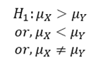
Let us suppose that two different concerns manufacture drugs for including sleep, drug A manufactured by first concern and drug B manufactured by second concern. Each company claims that its drug is superior to that of the other and it is desired to test which is a superior drug A or B? To formulate the statistical hypothesis let X be a random variable which denotes the additional hours of sleep gained by an individual when drug A is given and let the random variable Y denote the additional hours to sleep gained when drug B is used. Let us suppose that X and Y follow the probability distributions with means 𝜇𝑥 and 𝜇𝑌 respectively.
Here our null hypothesis would be that there is no difference between the effects of two drugs. Symbolically,
𝐻0: 𝜇𝑋 = 𝜇𝑌
Alternative Hypothesis
A statistical hypothesis which differs from the null hypothesis is called an Alternative Hypothesis, and is denoted by 𝐻1. The alternative hypothesis is not tested, but its acceptance (rejection) depends on the rejection (acceptance) of the null hypothesis. Alternative hypothesis contradicts the null hypothesis. The choice of an appropriate critical region depends on the type of alternative hypothesis, whether both-sided, one-sided (right/left) or specified alternative.
Alternative hypothesis is usually denoted by 𝐻1.
For example, in the drugs problem, the alternative hypothesis could be
Power Of Test
The null hypothesis 𝐻0 𝜃 = 𝜃0 is accepted when the observed value of test statistic lies the critical region, as determined by the test procedure. Suppose that the true value of 𝜃 is not 𝜃0, but another value 𝜃1, i.e. a specified alternative hypothesis 𝐻1 𝜃 = 𝜃1 is true. Type II error is committed if 𝐻0 is not rejected, i.e. the test statistic lies outside the critical region. Hence the probability of Type II error is a function of 𝜃1, because now 𝜃 = 𝜃1 is assumed to be true. If 𝛽 𝜃1 denotes the probability of Type II error, when 𝜃 = 𝜃1 is true, the complementary probability 1 − 𝛽 𝜃1 is called power of the test against the specified alternative 𝐻1 𝜃 = 𝜃1 . Power = 1-Probability of Type II error=Probability of rejection 𝐻0 when 𝐻1 is true Obviously, we could like a test to be as ‘powerful’ as possible for all critical regions of the same size. Treated as a function of 𝜃, the expression of 𝑃 𝜃 = 1 − 𝛽 𝜃 is called Power Function of the test for 𝜃0 against 𝜃. the curve obtained by plotting P(𝜃) against all possible values of 𝜃, is known as Power Curve.
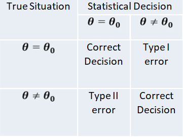
Elements: Type I & Type II Error
Type I Error & Type Ii Error
The procedure of testing statistical hypothesis does not guarantee that all decisions are perfectly accurate. At times, the test may lead to erroneous conclusions. This is so, because the decision is taken on the basis of sample values, which are themselves fluctuating and depend purely on chance. The errors in statistical decisions are two types:
Type I Error – This is the error committed by the test in rejecting a true null hypothesis.
Type II Error – This is the error committed by the test in accepting a false null hypothesis.
Considering for the population mean is 40, i.e. 𝐻0 𝜇 = 40 , let us imagine that we have a random sample from a population whose mean is really 40. if we apply the test for 𝐻0 𝜇 = 40 , we might find that the values of test statistic lines in the critical region, thereby leading to the conclusion that the population mean is not 40; i.e. the test rejects the null hypothesis although it is true. We have thus committed what is known as “Type I error” or “Error of first kind”. On the other hand, suppose that we have a random sample from a population whose mean is known to different from 40, say 43. if we apply the test for 𝐻0 𝜇 = 40 , the value of the statistic may, by chance, lie in the acceptance region, leading to the conclusion that the mean may be 40; i.e. the test does not reject the null hypothesis 𝐻0 𝜇 = 40 , although it is false. This is again another form of incorrect decision, and the error thus committed is known as “Type II error” or “Error of second kind”.
Using sampling distribution of the test statistic, we can measure in advance the probabilities of committing the two types of error. Since the null hypothesis is rejected only when the test statistic falls in the critical region.
Probability of Type I error = Probability of rejecting 𝐻0 𝜃 = 𝜃0 , when it is true = Probability that the test statistic lies in the critical region, assuming 𝜃 = 𝜃0.
The probability of Type I error must not exceed the level of significance (𝛼) of the test.
The probability of Type II error assumes different values for different values of 𝜃 covered by the alternative hypothesis 𝐻1. Since the null hypothesis is accepted only when the observed value of the best statistic lies outside the critical region.
Probability of Type II error 𝑊ℎ𝑒𝑛 𝜃 = 𝜃1 = Probability of accepting 𝐻0 𝜃 = 𝜃0 , when it is false = Probability that the test statistic lies in the region of acceptance, assuming 𝜃 = 𝜃1
The probability of Type I error is necessary for constructing a test of significance. It is in fact the ‘size of the Critical Region’. The probability of Type II error is used to measure the “power” of the test in detecting falsity of the null hypothesis. When the population has a continuous distribution
Probability of Type I error = Level of significance = Size of critical region
Elements: Level Of Significance & Critical Region
Level Of Significance And Critical Region
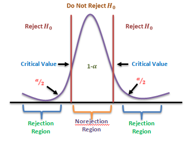
The decision about rejection or otherwise of the null hypothesis is based on probability considerations. Assuming the null hypothesis to be true, we calculate the probability of obtaining a difference equal to or greater than the observed difference. If this probability is found to be small, say less than .05, the conclusion is that the observed value of the statistic is rather unusual and has been caused due to the underlying assumption (i.e. null hypothesis) that is not true. We say that the observed difference is significant at 5 per cent level, and hence the ‘null hypothesis is rejected’ at 5 per cent level of significance. If, however, this probability is not very small, say more than .05, the observed difference cannot be considered to be unusual and is attributed to sampling fluctuation only. The difference is, now said to be not significant at 5 per cent level, and we conclude that there is no reason to reject the null hypothesis’ at 5 per cent level of significance. It has become customary to use 5% and 1% level of significance, although other levels, such as 2% or 5% may also be used.
Without actually going to calculate this probability, the test of significance may be simplified as follows. From the sampling distribution of the statistic, we find the maximum difference is which is exceeded in (say 5) percent of cases. If the observed difference in larger than this value, the null hypothesis is rejected. It is less there in no reason to reject the null hypothesis.
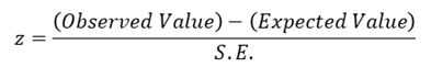
Suppose, the sampling distribution of the statistic is a normal distribution. Since the area under normal curve outside the ordinates at mean ±1.96 (𝑠. 𝑑. ) is only 5%, the probability that the observed value of the statistic differs from the expected value of 1.96 times the S.E. or more is .05; and the probability of a larger difference will be still smaller. If, therefore
Is either greater than 1.96 or less than -1.96 (i.e. numerically greater than 1.96), the null hypothesis 𝐻0 is rejected at 5% level of significance. The set values 𝑧 ≥ 1.96 𝑜𝑟 ≤ −1.96, i.e.
|𝑧| ≥ 1.96
constitutes what is called the Critical Region for the test. Similarly since the area outside mean ±2.58 (s.d.) is only 1%. 𝐻0 is rejected at 1% level of significance, if z numerically exceeds 258, i.e. the critical region is 𝑧 ≥ 2.58 at 1% level. Using the sampling distribution of an appropriate test statistic we are able to establish the maximum difference at a specified level between the observed and expected values that is consistent with null hypothesis 𝐻0 . The set of values of the test statistic corresponding to this difference which lead to the acceptance of 𝐻0 is called Region of acceptance. Conversely, the set of values of the statistic leading to the rejection of 𝐻0 is referred to as Region of Rejection or “Critical Region” of the test. The value of the statistic which lies at the boundary of the regions of acceptance and the rejection is called Critical value. When the null hypothesis is true, the probability of observed value of the test statistic falling in the critical region is often called the “Size of Critical Region”.
𝑆𝑖𝑧𝑒 𝑜𝑓 𝐶𝑟𝑖𝑡𝑖𝑐𝑎𝑙 𝑅𝑒𝑔𝑖𝑜𝑛 ≤ 𝐿𝑒𝑣𝑒𝑙 𝑜𝑓 𝑆𝑖𝑔𝑛𝑖𝑓𝑖𝑐𝑎𝑛𝑐𝑒
However, for a continuous population, the critical region is so determined that its size equals the Level of Significance (𝛼).
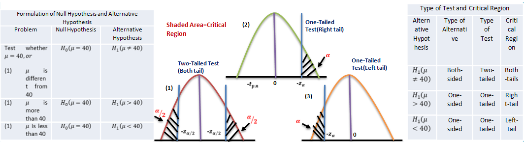
Two-Tailed And One-Tailed Tests
Our discussion above were centered around testing the significance of ‘difference’ between the observed and expected values, i.e. whether the observed value is significantly different from (i.e. either larger or smaller than) the expected value, as could arise due to fluctuations of random sampling. In the illustration, the null hypothesis is tested against “both-sided alternatives” 𝜇 > 40 𝑜𝑟 𝜇 < 40 , i.e.
𝐻0 𝜇 = 40 𝑎𝑔𝑎𝑖𝑛𝑠𝑡 𝐻1 𝜇 ≠ 40
Thus assuming 𝐻0 to be true, we would be looking for large differences on both sides of the expected value, i.e. in “both tails” of the distribution. Such tests are, therefore, called “Two-tailed tests”.
Sometimes we are interested in tests for large differences on one side only i.e., in one ‘one tail’ of the distribution. For example, whether a change in the production bricks with a ‘higher’ breaking strength, or whether a change in the production technique yields ‘lower’ percentage of defectives. These are known as “One-tailed tests”.
For testing the null hypothesis against “one-sided alternatives (right side)” 𝜇 > 40 , i.e.
𝐻0 𝜇 = 40 𝑎𝑔𝑎𝑖𝑛𝑠𝑡𝐻1 𝜇 > 40
The calculated value of the statistic z is compared with 1.645, since 5% of the area under the standard normal curve lies to the right of 1.645. if the observed value of z exceeds 1.645, the null hypothesis 𝐻0 is rejected at 5% level of significance. If a 1% level were used, we would replace 1.645 by 2.33. thus the critical regions for test at 5% and 1% levels are 𝑧 ≥ 1.645 and 𝑧 ≥ 2.33 respectively.
For testing the null hypothesis against “one-sided alternatives (left side)” 𝜇 < 40 i.e.
𝐻0 𝜇 = 40 𝑎𝑔𝑎𝑖𝑛𝑠𝑡𝐻1 𝜇 < 40
The value of z is compared with -1.645 for significance at 5% level, and with -2.33 for significance at 1% level. The critical regions are now 𝑧 ≤ −1.645 and 𝑧 ≤ −2.33 for 5% and 1% levels respectively. In fact, the sampling distributions of many of the commonly-used statistics can be approximated by normal distributions as the sample size increases, so that these rules are applicable in most cases when the sample size is ‘large’, say, more than 30. It is evident that the same null hypothesis may be tested against alternative hypothesis of different types depending on the nature of the problem. Correspondingly, the type of test and the critical region associated with each test will also be different.
Solving Testing Of Hypothesis Problem
Step 1 Set up the “Null Hypothesis” 𝐻0 and the “Alternative Hypothesis” 𝐻1 on the basis of the given problem. The null hypothesis usually specifies the values of some parameters involved in the population: 𝐻0 𝜃 = 𝜃0 . The alternative hypothesis may be any one of the following types: 𝐻1 ( ) 𝜃 ≠ 𝜃1 𝐻1 𝜃 > 𝜃0 , 𝐻1 𝜃 < 𝜃0 . The types of alternative hypothesis determines whether to use a two-tailed or one-tailed test (right or left tail).
Step 2
State the appropriate “test statistic” T and also its sampling distribution, when the null hypothesis is true. In large sample tests the statistic 𝑧 = (𝑇 − 𝜃0)Τ𝑆. 𝐸. , (T) which approximately follows Standard Normal Distribution, is often used. In small sample tests, the population is assumed to be Normal and various test statistics are used which follow Standard Normal, Chi-square, t for F distribution exactly.
Step 3 Select the “level of significance” 𝛼 of the test, if it is not specified in the given problem. This represents the maximum probability of committing a Type I error, i.e., of making a wrong decision by the test procedure when in fact the null hypothesis is true. Usually, a 5% or 1% level of significance is used (If nothing is mentioned, use 5% level).
Step 4
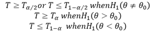
Find the “Critical region” of the test at the chosen level of significance. This represents the set of values of the test statistic which lead to rejection of the null hypothesis. The critical region always appears in one or both tails of the distribution, depending on weather the alternative hypothesis is one-sided or both-sided. The area in the tails must be equal to the level of significance 𝛼. For a one-tailed test, 𝛼 appears in one tail and for two-tailed test 𝛼/2 appears in each tail of the distribution. The critical region is
Where 𝑇𝛼 is the value of T such that the area to its tight is 𝛼.
Step 5
Compute the value of the test statistic T on the basis of sample data the null hypothesis. In large sample tests, if some parameters remain unknown they should be estimated from the sample. Step 6
If the computed value of test statistic T lies in the critical region, “reject 𝐻0”; otherwise “do not reject 𝐻0 ”. The decision regarding rejection or otherwise of 𝐻0 is made after a comparison of the computed value of T with critical value (i.e., boundary value of the appropriate critical region).
Step 7 Write the conclusion in plain non-technical language. If 𝐻0 is rejected, the interpretation is: “the data are not consistent with the assumption that the null hypothesis is true and hence 𝐻0 is not tenable”. If 𝐻0 is not rejected, “the data cannot provide any evidence against the null hypothesis and hence 𝐻0 may be accepted to the true”. The conclusion should preferably be given in the words stated in the problem.
Conclusion
Hypothesis is a statistical statement or a conjecture about the value of a parameter. The legal concept that one is innocent until proven guilty has an analogous use in the world of statistics. In devising a test, statisticians do not attempt to prove that a particular statement or hypothesis is true. Instead, they assume that the hypothesis is incorrect (like not guilty), and then work to find statistical evidence that would allow them to overturn that assumption. In statistics this process is referred to as hypothesis testing, and it is often used to test the relationship between two variables. A hypothesis makes a prediction about some relationship of interest. Then, based on actual data and a pre-selected level of statistical significance, that hypothesis is either accepted or rejected. There are some elements of hypothesis like null hypothesis, alternative hypothesis, type I & type II error, level of significance, critical region and power of test and some processes like one and two tail test to find the critical region of the graph as well as the error that help us reach the final conclusion.
A Null hypothesis is a hypothesis that says there is no statistical significance between the two variables in the hypothesis. There is no difference between certain characteristics of a population. It is denoted by the symbol 𝐻0. A statistical hypothesis which differs from the null hypothesis is called an Alternative Hypothesis, and is denoted by 𝐻1. The procedure of testing statistical hypothesis does not guarantee that all decisions are perfectly accurate. At times, the test may lead to erroneous conclusions. This is so, because the decision is taken on the basis of sample values, which are themselves fluctuating and depend purely on chance, this process called types of error. Hypothesis testing is very important part of statistical analysis. By the help of hypothesis testing many business problem can be solved accurately.
That was the fourth part of the series, that explained hypothesis testing and hopefully it clarified your notion of the same by discussing each crucial aspect of it. You can find more informative posts like this one on Data Science course topics. Just keep on following the Dexlab Analytics blog to stay informed.
Here is taking an in-depth look at how sampling distribution works along with a discussion on various types of the sampling distribution. This is a continuation of the discussion on Classical Inferential Statistics that focused on the theory of sampling, breaking it down to building blocks of classical sampling theory along with various kinds of sampling. You can read part 1 of the article here
The sampling distribution is a probability distribution of statistics obtained from a large number of samples drawn from a specific population. And the types of sampling distribution are- (i) Gamma Distribution, (ii) Beta Distribution, (iii) Chi-Square Distribution, (iv) Exponential Distribution, (v) T-Distribution & (vi) F-Distribution.
The key components for describing all these distributions are – (i) Probability Density Function – Which is the function whose integral is to be calculated to find probabilities associated with a continuous random variable and their shape(graph) for the same, (ii) Moment Generating Function – which helps to find the moment of those distributions, and (iii) Degrees of Freedom – It refers to the number of independent sample points and compute a static minus the number of parameters explained from the sample.
For Gamma and Beta distribution, we will discuss gamma and beta function and relation between them etc.
2. Probability Density Function, Moment Generating Function, Sampling Distribution, Degrees of Freedom
PROBABILITY DENSITY FUNCTION
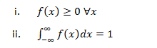
Probability density function (PDF), in statistics, is a function whose integral is calculated to find probabilities associated with a continuous random variable (see continuity; probability theory). Its graph is a curve above the horizontal axis that defines a total area, between itself and the axis, of 1. The percentage of this area included between any two values coincides with the probability that the outcome of an observation described by the probability density function falls between those values. Every random variable is associated with a probability density function (e.g., a variable with a normal distribution is described by a bell curve). If X be continuous Random variable taking any continuous real values then f(x) is a probability density function if:-
Moment Generating Function
The moment generating function (m.g.f.) of a random variable X (about origin) having the probability function f(x) is given by:
The integration of summation being extended to the entire range of x, t being the real parameter and it is being assumed that the right-hand side of the equation is absolutely convergent for some positive number h such that –h<t<h.
SAMPLING DISTRIBUTION
It may be defined as the probability law which the statistic follows if repeated random samples of a fixed size are drawn from a specified population. A number of samples, each of size n, are taken from the same population and if for each sample the values of the statistic are calculated, a series of values of the statistic will be obtained. If the number of samples is large, these may be arranged into a frequency table. The frequency distribution of the statistic that would be obtained if the number of samples, each of the same size (say n), were infinite is called the Sampling distribution of the statistic
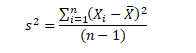
DEGREES OF FREEDOM
The term degrees of freedom (df) refers to the number of independent sample points used to compute a statistic minus the number of parameters estimated from the sample points: For example, consider the sample estimate of the population variance (s2)
Where is the score for observation i in the sample, X ̅ is the sample estimate of the population mean, n is the number of observation in the sample. The formula is based on n independent sample points and one estimated population parameter (x ̅). Therefore, the number of degrees of freedom is n minus one. For this example
df=n-1
3. Gamma Function, Beta Function, Relation between Gamma &Beta Function
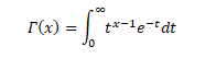
GAMMA FUNCTION
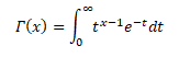
The Gamma function is defined for x>0 in integral form by the improper integral known as Euler’s integral of the second kind.
Many probability distributions are defined by using the gamma function, such as gamma distribution, beta distribution, chi-squared distribution, student’s t-distribution, etc. For data scientists, machine learning engineers, researchers, the Gamma function is probably one of the most widely used functions because it is employed in many distributions.
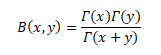
BETA FUNCTION
The Beta function is a function of two variables that is often found in probability theory and mathematical statistics.
The Beta function is a function B: R_(++)^2→R defined as follows:
There is also a Euler’s integral of the first kind.
For example, as a normalizing constant in the probability density functions of the F distribution and of the Student’s t distribution
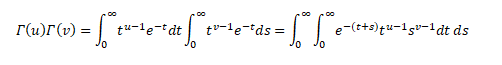
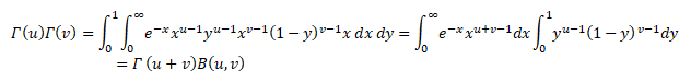
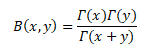
RELATION BETWEEN GAMMA AND BETA FUNCTION
In the realm of Calculus, many complex integrals can be reduced to expressions involving the Beta Function. The Beta Function is important in calculus due to its close connection to the Gamma Function which is itself a generalization of the factorial function.
We know,
So, the product of two factorials as
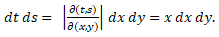
Now apply the changes of variables t=xy and s=x(1-y) to this double integral. Note that t + s = x and that 0 < t < ∞ and 0 < x < ∞ and 0 < y < 1. The jacobian of this transformation is
Since x > 0 we conclude that Hence we have
Therefore,
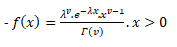
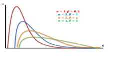
4. Gamma Distribution
The gamma distribution is a widely used distribution. It is a right-skewed probability distribution. These distributions are useful in real life where something has a natural minimum of 0.
If X be a continuous random variable taking only positive values, then X is said to be following a gamma distribution iff its p.d.f can be expressed as:-
=0 otherwise….(1)
Probability Density Function for Gamma Distribution
For (1), to be the Probability Density Function, we must have:-
Now, f(x)>0 if x>0 & f(x)=0 if x taking any non-positive values, so, f(x)≥0 ∀x .
Hence, condition (i) is satisfied. Now,
Using (3) & (4) in (2) we get:-
Hence, f(x) statistics condition (ii).
So, equation (1) is a proper pdf.
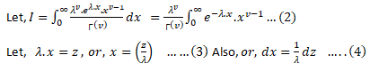
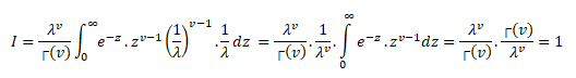
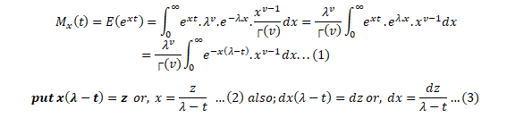
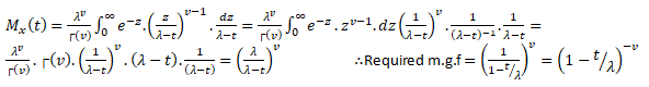
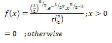
Moment Generating Function for Gamma Distribution
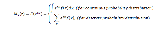
Moment generating functions are general procedure of finding out moments of a probability distribution mathematically it may be expressed as- M_x (t)=E(e^xt )
This represents raw moments of the random variable X about to the origin 0.
Three important properties of m.g.f. are:- (i) where c is a constant.(ii) If ’s are independent Random variables i.e. then (iii) If X and Y are two random variables and if then X and Y are two identical distribution this is called the uniqueness property,Calculating the m.g.f. of gamma distribution:
Using (2) and (3) in (1) we get:
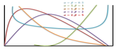
5. Beta Distribution
In probability theory and statistics, the beta distribution is a family of continuous probability distributions defined on the interval [0, 1] parameterized by two positive shape parameters, denoted by α and β, that appear as exponents of the random variable and control the shape of the distribution.
The beta distribution has been applied to model the behavior of random variables limited to intervals of finite length in a wide variety of disciplines.
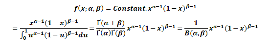
Probability Density Function for Beta Distribution
The probability density function (PDF) of the beta distribution, for 0 ≤ x ≤ 1, and shape parameters α, β > 0, is a power function of the variable x and of its reflection (1 − x) as follows:
Where Γ(z) is the gamma function. The beta function, B, =+is a normalization constant to ensure that the total probability integrates to 1. In the above equations, x is a realization—an observed value that actually occurred—of a random process X.
This definition includes both ends x = 0 and x = 1, which is consistent with the definitions for other continuous distributions supported on a bounded interval which are special cases of the beta distribution, for example, the arcsine distribution, and consistent with several authors, like N. L. Johnson and S. Kotz. However, the inclusion of x= 0 and x= 1 does not work for α, β < 1; accordingly, several other authors, including W. Feller, choose to exclude the ends x = 0 and x = 1, (so that the two ends are not actually part of the domain of the density function) and consider instead 0 < x < 1. Several authors, including N. L. Johnson and S. Kotz, use the symbols p and q (instead of α and β) for the shape parameters of the beta distribution, reminiscent of the symbols are traditionally used for the parameters of the Bernoulli distribution, because the beta distribution approaches the Bernoulli distribution in the limit when both shape parameters α and β approach the value of zero.
In the following, a random variable X beta-distributed with parameters α and β will be denoted by:
Other notations for beta-distributed random variables used in the statistical literature are. X- Be(α,β)and X~β_(α,β)
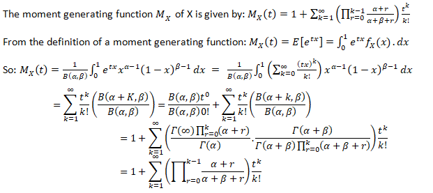
Moment Generating Function for Beta Distribution
6. Chi-square Distribution & Exponential Distribution
CHI-SQUARE DISTRIBUTION
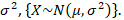
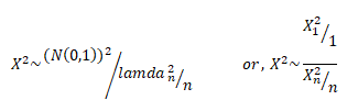
A chi-square distribution is defined as the sum of the squares of standard normal variates. Let x be a random variable which follows normal distribution with mean μ& variance then standard normal variate is defined as: –
The variate Z is said to follow a standard normal distribution with mean 0 and variance 1. Let X be a random variable containing observations,.
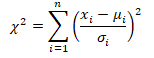
Then the chi-square distribution is defined as:- So we can say:-
A chi-square distribution with ‘n’ degree of freedom, where degrees of freedom refer to number of independent associations among variables.
The Probability Density Function of a Chi-Square Distribution:
The Moment Generating Function of Chi-Square Distribution:
(4) is a required m.g.f. of the chi-square distribution.
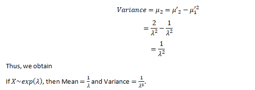
EXPONENTIAL DISTRIBUTION
The Exponential distribution is one of the widely used continuous distributions. It is often used to model the time elapsed between events.
The Probability Density Function of Exponential Distribution:
Let X be a continuous random variable assuming only real values then X is said to be following an exponential distribution iff:-
Therefore, exponential distribution is a special case of gamma
distribution with v = 1.
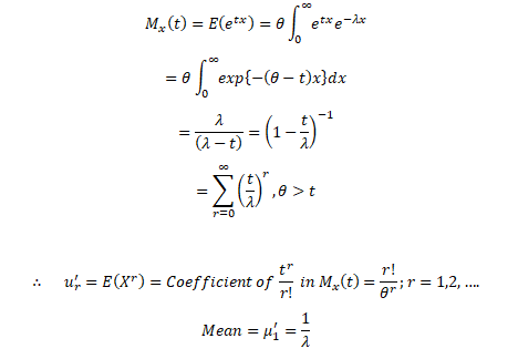
The Moment Generating Function of Exponential Distribution:
Let X~Exponential (λ), we can find its expected value as follows, using integration by parts:
Now let’s find Var (X), we have
7. T-Distribution & F-Distribution
T-DISTRIBUTION
Student’s t-distribution:
If x1,x2,… ,xn be ‘n’ random samples drawn from a normal population having mean & standard deviation then the statistics following student t-distribution with (n-1) degrees of freedom.
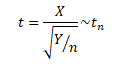
Fisher’s t-distribution:
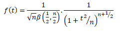
Let X~N(0,1) & let the random variable Y~X_n^2. Both X & Y are independent random variables. Then the fisher’s t-distribution is defined as :-
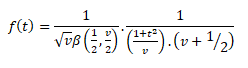
Probability Density Function for t-distribution:
Where, t2 > 0 Where, v=(n-1) degrees of freedom
= 0 , otherwise
For Fisher’s t-distribution:
Where, t2 > 0
=0 otherwise
Application of t-distribution:
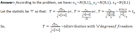
If x1,x2, and x3 are independent random variables. Each following a standard normal distribution. What will be the distribution of
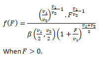
F- DISTRUBUTION
The F-Distribution is a ration of two chi-square distributions. If X be a random variable which follows a fisher’s t-distribution.Then:-
Squaring the above expression we get:
The R.V. X2~F1, n. Then we say X2 follows F-distribution with 1,n degrees of freedom.
Probability Density Function for F-distribution:
Application of F-Distribution:
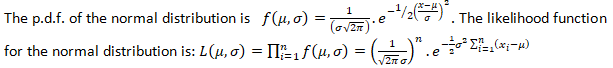
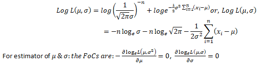
Let x1,x2,… ,xn be a random sample drawn from a normal population with mean μ & variance σ2. where both μ & σ are unknown. Obtain the MLEs of θ.
Let x1,x2,… ,xn be ‘n’ random sample drawn from a normal population with mean μ & variance σ2.
Taking logarithms on both sides; we get:-
CONCLUSION: That was a thorough analysis of different types of sampling distribution along with their distinct functions and interrelations. If the resource was useful in understanding statistical analytics, find more such informative and analytical, subject-oriented discussion regarding statistical analytics courses on DexLab Analytics blog.
Indian IT sector is expected to grow at a modest rate this fiscal year, which started from April – companies are expanding their scopes and building new capabilities or enhancing the older ones. Demand for digital services is showing spiked up trends. The good news is that the digital component industry is flourishing, faster than expected. It’s forming a bigger part of tech-induced future, and we’re all excited!!
On that positive note, here we’ve culled down a few fun facts about IT industry that are bound to intrigue your data-hungry heart and mind… Hope you’ll enjoy the read as much as I did while scampering through research materials to compile this post!
Let’s get started…
Email is actually older than the World Wide Web.
Our very own, Hewlett Packard started in a garage… In fact, several other top notch US digital natives, including Microsoft, Google and Apple had such humble beginnings.
Bill Gates’ own house was designed using a MAC PC, yes you heard that right!
The very first computer mouse was carved out of wood. Invented by Dough Engelbart, first-ever mouse wasn’t made of any plastic or metal of any kind, but plain, rustic WOOD.
The QWERTY keyboard, which we use now, is simple, easy to use and effective. But, did you know: DVORAK keyboard was proven to be at least 20X faster?
The original name of Windows OS was Interface Manager.
Do you think 1GigaByte is enough? Well, the first 1 GB hard drive made news in 1980 with a price tag of $40.000 and gross weight of 550 pounds.
Very first PC was known as ‘Simon’ from Berkley Enterprise. It was worth $300, which was quite an ostentatious amount back in the 1950s, the year when this PC was launched.
In 1950’s computers were called ‘Electronic Brains’.
1 out of 8 marriages in the US happened between couples who’ve met online. Wicked?
Feeling excited to know all these stuffs… Now, on serious note, in the days to come, the Indian IT industry is all set to transform itself with high velocity tools and technology, and if you want to play a significant role in this digital transformation, arm yourself with decent data-friendly skill or tool.
The deal turns sweeter if you hail from computer science background or have a knack to play with numbers. If such is the case, we have high end business analyst training courses in Gurgaonto suit your purpose and career aspiration – drop by DexLab Analytics, being a top of the line analytics training institute, they bring to you a smart concoction of knowledge, aptitude and expertise in the form of student-friendly curriculum. For more details, visit their site today.
To learn more about Data Analyst with Advanced excel course – Enrol Now. To learn more about Data Analyst with R Course – Enrol Now. To learn more about Big Data Course – Enrol Now.
To learn more about Machine Learning Using Python and Spark – Enrol Now. To learn more about Data Analyst with SAS Course – Enrol Now. To learn more about Data Analyst with Apache Spark Course – Enrol Now. To learn more about Data Analyst with Market Risk Analytics and Modelling Course – Enrol Now.
According to Google Search, ‘blockchain’ is defined as “a digital ledger in which transactions made in bitcoin or in other cryptocurrency is recorded chronologically and publicly.”
Speaking in a way of cryptocurrency, a block is a record of new transactions that could mean the actual location of cryptocurrency. Once each block has completed its transaction, it’s added to the chain, creating a chain of blocks known as blockchain.
Suppose a Google spreadsheet is shared by each and every computer which is connected to the internet in this world. When a transaction happens, it will be recorded in a row of this spreadsheet. Just like a spreadsheet has rows, Blockchain consists of Blocks for each transaction.
Whoever has access to a computer or mobile can connect to the internet and can have access to the spreadsheet and add a transaction, but the spreadsheet doesn’t permit anyone to edit the information which is already available. No third party can interfere into its transactions, therefore saves time and conflict.
Types of Blockchains:
Open and permission-less: Public and permissionless blockchains look like bitcoin, the first blockchain. All exchanges in these blockchains are open and no authorizations are required to join these circulated elements.
Private and permission: These blockchains are constrained to assigned individuals, exchanges are private, and authorization from a proprietor or supervisor substance is required to join this system. These are frequently utilized by private consortia to oversee industry esteem chain openings.
Hybrid blockchains: An extra region is a developing idea of sidechain, which takes into consideration distinctive blockchains (open or private) to speak with each other, empowering exchanges between members crosswise over blockchain systems.
Various Applications Of Blockchain Are As Follows:
a) Smart Contracts:
Smart Contracts eases the way we exchange money, property, shares and avoids third person/party conflicts. Smart keys access can only be permitted to the authorized party. Basically, computers are given the command to control the contracts and to release or hold the funds by giving the keys to the permitted persons.
For example, if I want to rent an office space from you, we can do this in blockchain using cryptocurrency. You will get a receipt which is saved in the virtual contract and I will get the digital entry key which will reach me by a specified date. If you send the key before the specified date, the function holds it and releases both receipt and the key when the date arrives.
If I receive the key I surely should pay you. And this contract will be canceled when the time gets complete, and it cannot interfere as all the participants will be alerted. The Smart contracts can be used for insurance premiums, financial derivatives, financial services, legal processes etc.
b) Digital Identity:
The future of blockchain will be blooming in the coming years. Blockchain technologies make both managing and tracking digital identities reliable and systematic, resulting in easy registering and minimizing fraud.
Be it national security, citizenship documentation, banking, online retailing or healthcare, identity authentication and authorization is a process entangled in between commerce and culture, worldwide. Introducing blockchain into identity-based mechanisms can really bring captivating solutions to the security problems we have online.
Blockchain technology is known to offer a solution to many digital identity issues, where identity can be uniquely validated in an undeniable, unchangeable, and secured manner.
Present-day methods involve problematic password-based systems of known secrets which are exchanged and stored on insecure computer systems. Blockchain-based certified systems are actually built on undeniable identity verification for using digital signatures based on the public key related cryptography.
In blockchain identity confirmation, the only check that is performed is to know if the transaction was signed by the authorized private key. It is implied to whoever has access to the private key is the owner and the exact identity of the owner is deemed unrelated.
c) Insurance:
Claims dealing can be disappointing and unrewarding. Insurance agents need to go through deceitful cases and deserted approaches, or divided information sources for clients to express a few – and process these documents manually. Space for mistake is enormous. The blockchain gives an ultimate framework for hazard-free administration and clarity. Its encryption properties enable insurers to represent the ownership to be protected.
“This will be the toughest on the portions of the industry that are least differentiated, where consumers often decide based on price: auto, life, and homeowner’s insurance.” — Harvard Business Review
d) Supply-Chain Communications and Proof-of-Provenance:
The majority of the things we purchase aren’t made by a single organization, yet by a chain of providers who offer their ingredients (e.g., graphite for pencils) to an organization that gathers and markets the final commodity. On the off chance that any of those commodities flops, in any case, the brand takes the brunt of the backfire — it holds most of the duty regarding its supply chain network.
However, consider the possibility that an organization could proactively give carefully perpetual, auditable records that show stakeholders the condition of the item at each esteem included process.
This is not a little task: The worldwide supply chain network is evaluated to be worth $40 trillion; and from a business-process point of view, it’s a fabulously incapable chaos. As a related issue, blockchain can be utilized to track diamonds, creative skill, real estate, and practically any other resources.
e) Music Industry:
While music lovers have hailed digitization as the popular government of the music business, 15.7 billion dollar music industry is confusingly continuing as before. Music piracy through unlawfully downloaded, duplicated and shared content eats into the artist’s sovereignties and music labels’ income. Added to this, is the absence of a vigorous rights administration framework, which prompts loss of income to the artist.
Also, the income, when it really achieves the artist, can take up to two years! Another region of concern is unpaid sovereignties, which are frequently suspended in different stages because of missing data or rights possession. There is additionally an absence of access to continuous advanced sales information, which if accessible can be utilized to strategize advertising efforts more successfully.
These very zones are the place Blockchain can have stunning effects. As a publically accessible and decentralized database that is distributed over the web, Blockchain keeps up lasting and undeletable records in cryptographic format. Exchanges happen over a peer to peer system and are figured, confirmed and recorded utilizing a computerized agreement strategy, disposing of the requirement for an intermediator or outsider to oversee or control data.
The very engineering of Blockchain being unchanging, dispersed and distributed conveys enormous potential to manage the present troubles influencing the music business.
An essential region in which Blockchain can bring out positive change is in the formation of a digital rights database. Digital rights articulation is one of the basic issues distressing the present music industry. Recognizing copyright of a melody and characterizing how sovereignties ought to be part of musicians, entertainers, distributors, and makers are troublesome in digital space. Regularly artists miss out on sovereignties because of complicated copyright condition.
Blockchain’s changeless distributed ledger framework, which guarantees that no single organization can assert proprietorship, ensures an ideal arrangement. Secure documents with all applicable data, for example, structure, versus, straight notes, cover craftsmanship, permitting, and so on, can be encoded onto the Blockchain making a changeless and inerasable record.
f) Government and Public records:
The administration of public services is yet another region, where blockchain can help diminish paper-based procedures, limit fraud, and increment responsibility amongst specialists and those they serve.
Some US states are volunteering to understand the advantages of blockchain: the Delaware Blockchain Initiative propelled in 2016, expects to make a proper legitimate foundation for distributed ledger shares to increase productivity and speed of consolidation administrations.
Illinois, Vermont, and different states have since reported comparative activities. Startup companies are sponsoring in the effort also: in Eastern Europe, the BitFury Group is presently working with the Georgian government to secure and track government records.
Conclusion:
This article focused on the blockchain and its applications in various industries explains challenges and potentials and how people can secure their information digitally without any issues and increasing their ability. As these applications are still under development and yet to be untangled in the future, blockchain could become a powerful tool conducting fair trade, improving business and supporting the society.
K.Maneesha is an SEO Developer At Mindmajix.com. She holds a masters degree in Marketing from Alliance University, Bangalore. Maneesha is a dog-lover and enjoys traveling with friends on trips. You can reach her at manisha.m4353@gmail.com. Her LinkedIn profile Maneesha Kakulapati.
Interested in a career in Data Analyst?
To learn more about Machine Learning Using Python and Spark – click here.
To learn more about Data Analyst with Advanced excel course – click here. To learn more about Data Analyst with SAS Course – click here. To learn more about Data Analyst with R Course – click here. To learn more about Big Data Course – click here.
Business Intelligence, or BI, is crucial for organizations as strategic planning is heavily dependent on BI. BI tools are multi-purpose and used for indicating progress towards business goals, quantitatively analyzing data, distribution of data and developing customer insights.
Advanced computer technologies are applied in Business Intelligence to discover relevant business data and then analyze it. It not only spots current trends in data, but is also able to develop historical views and future predictions. This helps decision-makers to comprehend business information properly and develop strategies that will steer their organization forward.
BI tools transform raw business information into valuable data that increase revenue for organizations. The global business economy is completely data driven. Companies without BI software will be jeopardizing their success. It is time to shed the belief that BI software is superfluous. Rather, it is a necessity.
Here is a list of 10 important things that BI solutions can help your organization achieve. After reading these you will be convinced that BI is vital in taking your business forward.
Provide speedy and competent information for your business
Nowadays, there isn’t much time to ponder over data sheets and then come to a conclusion. Decisions have to be taken on the spot. Valuable information doesn’t include business data alone, but also what the data implies for your business. BI gives you a competitive lead as it provides valuable information with the push of a button.
Provide KPIs that boost the performance of your business.
Business Intelligence software provides KPIs (Key Performance Indicators), which are metrics aligned with your business strategies. Thus, businesses can make decisions based on solid facts instead of intuition. This makes business proceedings more efficient.
Employees have data-power
BI solutions help employees to make informed decisions backed by relevant data. Access to information across all levels ensures company-wide integration of data. This helps employees nurture their skills. A competitive workforce will help a company gain global recognition.
Determine the factors that generate revenue for your business
Business intelligence is able to determine where and how potential customers consume data, how to convert them to paying customers, and chalk out an appropriate plan that will help increase revenue for your business.
Avoid blockages in markets
There are many BI applications that can be incorporated with accounting software. Business intelligence provides information about the real health of an organization, which cannot be determined from a profit and loss sheet. BI includes predictive features that help avoid blockages in markets and determine the right time for important decisions, like hiring new employees. Easy-to understand dashboards enable decision-makers to stay informed.
Create an efficient business model
As explained by Jeremy Levi, Director of Marketing, MarsWellness.com, ‘’ Why is BI more important than ever? In one word: oversaturation. The internet and the continued growth of e-commerce have saturated every market…For business owners, this means making smart decisions and trying to know where to put your marketing dollars and where to invest in infrastructure. Business intelligence lets you do that, and without it, you’re simply fumbling around for the light switch in the dark.”
Improved customer insights
In the absence of BI tools, one can spend hours trying to make sense out of previous reports without coming to a satisfactory conclusion. It is crucial for businesses to meet customer demands. BI tools help map patterns in customer behavior so businesses can prioritize loyal customers and improve customer satisfaction.
Helps save money
BI tools help spot areas in your business where costs can be minimized. For example, there is unnecessary spending occurring in the supply chain. BI can identify whether it is inefficient acquisition or maintenance that is translating to increased costs. Thus, it enables businesses to take the necessary actions to cut costs.
Improve efficiency of workers
Business intelligence solutions can monitor the output of members and functioning of teams. These help improve efficiency of the workers and streamline the business processes.
Protects businesses from cyber threats
Cyber crimes like data breaches and malware attacks are very common. Cyber security has become the need of the hour. Businesses should invest in BI solutions equipped with security tools that help protect their valuable data from hackers and other cyber attacks.
Businesses will progress rapidly through the use of smart BI solutions. Organizations small or big, can use BI tools in a variety of areas, starting from budgets to building relationship with customers.
If you want to empower your business through BI then enroll yourself for the Tableau BI certification course at DexLab Analytics, Delhi. DexLab is a premium institute providing business analysis trainingin Delhi.
Interested in a career in Data Analyst?
To learn more about Machine Learning Using Python and Spark – click here. To learn more about Data Analyst with Advanced excel course – click here. To learn more about Data Analyst with SAS Course – click here. To learn more about Data Analyst with R Course – click here. To learn more about Big Data Course – click here.
To get valuable insights from the enormous quantity of data generated, credit unions need to move towards enterprise integration of data. This is a company-wide data democratization process that helps all departments within the credit union to manage and analyze their data. It allows each team member easy-access and proper utilization of relevant data.
However, awareness about the advantages of enterprise-wide data analytics isn’t sufficient for credit unions to deploy this system. Here is a three step guide to help credit unions get smarter in data handling.
Improve the quality of data
A robust and functional customer data set is of foremost importance. Unorganized data will hinder forming correct opinions about customer behavior. The following steps will ensure that relevant data enters the business analytics tools.
Integration of various analytics activity- Instead of operating separate analytics software for digital marketing, credit risk analytics, fraud detection and other financial activities, it is better to have a centralized system which integrates these activities. It is helpful for gathering cross-operational cognizance.
Experienced analytics vendors should be chosen- Vendors with experience can access a wide range of data. Hence, they can deliver information that is more valuable. They also provide pre-existing integrations.
Consider unconventional sources of data- Unstructured data from unconventional sources like social media and third-parties should be valued as it will prove useful in the future.
Continuous data cleansing that evolves with time- Clean data is essential for providing correct data. The data should be organized, error-free and formatted.
Data structure customized for credit unions
The business analytics tools for credit unions should perform the following analyses:
Analyzing the growth and fall in customers depending on their age, location, branch, products used, etc.
Measure the profit through the count of balances
Analyze the Performances of the staffs and members in a particular department or branch
Sales ratios reporting
Age distribution of account holders in a particular geographic location.
Perform trend analysis as and when required
Analyze satisfaction levels of members
Keep track of the transactions performed by members
Track the inquires made at call centers and online banking portals
Analyze the behavior of self-serve vs. non-self serve users based on different demographics
Determine the different types of accounts being opened and figure out the source responsible for the highest transactions.
User-friendly interfaces for manipulating data
Important decisions like growing revenue, mitigating risks and improving customer experience should be based on insights drawn using analytics tools. Hence, accessing the data should be a simple process. These following user-interface features will help make data user-friendly.
Dashboards- Dashboards makes data comprehensible even for non-techies as it makes data visually-pleasing. It provides at-a glance view of the key metrics, like lead generation rates and profitability sliced using demographics. Different datasets can be viewed in one place.
Scorecards- A scorecard is a type of report that compares a person’s performance against his goals. It measures success based on Key Performance Indicators (KPIs) and aids in keeping members accountable.
Automated reports- Primary stakeholders should be provided automated reports via mails on a daily basis so that they have access to all the relevant information.
Data analytics should encompass all departments of a credit union. This will help drawing better insights and improve KPI tracking. Thus, the overall performance of the credit union will become better and more efficient with time.
To learn more about Machine Learning Using Python and Spark – click here. To learn more about Data Analyst with Advanced excel course – click here. To learn more about Data Analyst with SAS Course – click here. To learn more about Data Analyst with R Course – click here. To learn more about Big Data Course – click here.
Moving to the cloud takes time. One of our friends started with Salesforce in 2009, after 5 years they introduced G Suite (widely known as Google Apps during that time) and it’s now in 2017 that they have adopted a fully cloud-based electronic health record facility. It took 10 years for an organization to resort to a handful number of installed applications for smooth handling of specialized tasks.
Nevertheless, their shift to Software-as-a-Service (SaaS) has had an impact on IT spending. Though the expenditure varies from company to company, every organization must have experienced these 5 changes highlighted below:
Better networks
Unsurprisingly, people need and expect faster internet speed these days. Even small businesses have connections that deliver 250Mbps down and 75Mbps (or more) up. An interesting switch is being observed in infrastructure. Today, more or less any medium-organization boasts of 802.11n or 802.11ac WIFI networks, which was unimaginable even few years ago. Deploying wireless mesh devices has become the order of the day now.
Lesser computer upgrades
There was a time, when we used to think that we have to replace our computers every three or five years. In several cases, we had even planned to make a few upgrades to the hardware to keep them running (RAM and hard-drive replacement was a common thought).
But in reality, organizations seldom have to replace parts. In most offices, five year old desktops perform perfectly in delivering the right results. This means definitely days of upgrades are over, all that matters is a faster internet speed and robust app development.
More usage of “plug-in and use” systems
More and more companies are seeking so-called “sealed” systems. Though some big companies still go on deploying standardized drive images, but increasingly organizations are found picking off-the-shelf sealed devices, like all-in-one desktops and non-use-configurable laptops.
As organizations are moving towards SaaS, Chromebooks are becoming increasingly famous. In fact, more than 20% of the team mentioned in the beginning of the blog uses a Chromebook as their primary work device.
Longer life for devices
Devices, like desktops and laptops that have embraced SaaS seem to have a longer lifecycle. As SaaS mostly depends on browser and network performance, the need for replacing devices has decreased to a great extent. Systems work totally until the device fails to perform or no longer in a position to receive any updates. Also, with SaaS, crucial data don’t remain solely on the device, hence if a system fails, little seems to be lost.
Considerable attention to the peripherals
Peripherals are intimidating. A large number of conventional desktop units have a scanner, printer and copier devices that are supported by a locally installed Windows software or server. Organizations can easily find alternatives of these devices, but it will take some time and effort as well. Few applications and sectors still suffer from minor or significant glitches, but over time, we hope peripherals and accessories will start showing signs of improvements.
What changes have you noticed in cloud computing and storage? How do you think the landscape of IT has changed over the past decade?
To learn more about Machine Learning Using Python and Spark – click here.
To learn more about Data Analyst with Advanced excel course – click here. To learn more about Data Analyst with SAS Course – click here. To learn more about Data Analyst with R Course – click here. To learn more about Big Data Course – click here.


 K.Maneesha is an SEO Developer At