Big Data Analytics Archives - DexLab Analytics | Big Data Hadoop SAS R Analytics Predictive Modeling & Excel VBA

Autocorrelation- Time Series – Part 3

Autocorrelation is a special case of correlation. It refers to the relationship between successive values of the same variables .For example if an individual with a consumption pattern:-
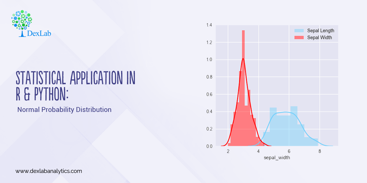
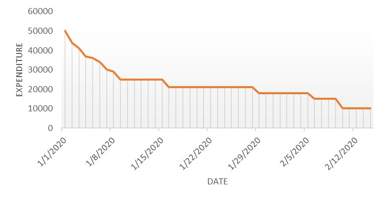
spends too much in period 1 then he will try to compensate that in period 2 by spending less than usual. This would mean that Ut is correlated with Ut+1 . If it is plotted the graph will appear as follows :

Positive Autocorrelation : When the previous year’s error effects the current year’s error in such a way that when a graph is plotted the line moves in the upward direction or when the error of the time t-1 carries over into a positive error in the following period it is called a positive autocorrelation.
Negative Autocorrelation : When the previous year’s error effects the current year’s error in such a way that when a graph is plotted the line moves in the downward direction or when the error of the time t-1 carries over into a negative error in the following period it is called a negative autocorrelation.

Now there are two ways of detecting the presence of autocorrelation
By plotting a scatter plot of the estimated residual (ei) against one another i.e. present value of residuals are plotted against its own past value.

If most of the points fall in the 1st and the 3rd quadrants , autocorrelation will be positive since the products are positive.

If most of the points fall in the 2nd and 4th quadrant , the autocorrelation will be negative, because the products are negative.
By plotting ei against time : The successive values of ei are plotted against time would indicate the possible presence of autocorrelation .If e’s in successive time show a regular time pattern, then there is autocorrelation in the function. The autocorrelation is said to be negative if successive values of ei changes sign frequently.
First Order of Autocorrelation (AR-1)
When t-1 time period’s error affects the error of time period t (current time period), then it is called first order of autocorrelation.
AR-1 coefficient p takes values between +1 and -1
The size of this coefficient p determines the strength of autocorrelation.
A positive value of p indicates a positive autocorrelation.
A negative value of p indicates a negative autocorrelation
In case if p = 0, then this indicates there is no autocorrelation.
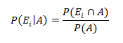
To explain the error term in any particular period t, we use the following formula:-

Where Vt= a random term which fulfills all the usual assumptions of OLS
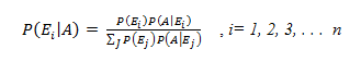
How to find the value of p?

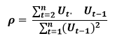
One can estimate the value of ρ by applying the following formula :-

Time Series Analysis & Modelling with Python (Part II) – Data Smoothing

dexlab_time_series

Data Smoothing is done to better understand the hidden patterns in the data. In the non- stationary processes, it is very hard to forecast the data as the variance over a period of time changes, therefore data smoothing techniques are used to smooth out the irregular roughness to see a clearer signal.

In this segment we will be discussing two of the most important data smoothing techniques :-

  • Moving average smoothing
  • Exponential smoothing

Moving average smoothing

Moving average is a technique where subsets of original data are created and then average of each subset is taken to smooth out the data and find the value in between each subset which better helps to see the trend over a period of time.

Lets take an example to better understand the problem.

Suppose that we have a data of price observed over a period of time and it is a non-stationary data so that the tend is hard to recognize.

QTR (quarter)Price
110
211
318
414
515
6?


In the above data we don’t know the value of the 6th quarter.

….fig (1)

The plot above shows that there is no trend the data is following so to better understand the pattern we calculate the moving average over three quarter at a time so that we get in between values as well as we get the missing value of the 6th quarter.

To find the missing value of 6th quarter we will use previous three quarter’s data i.e.

MAS =  = 15.7

QTR (quarter)Price
110
211
318
414
515
615.7

MAS =  = 13

MAS =  = 14.33

QTR (quarter)PriceMAS (Price)
11010
21111
31818
41413
51514.33
615.715.7


….. fig (2)

In the above graph we can see that after 3rd quarter there is an upward sloping trend in the data.

Exponential Data Smoothing

In this method a larger weight ( ) which lies between 0 & 1 is given to the most recent observations and as the observation grows more distant the weight decreases exponentially.

The weights are decided on the basis how the data is, in case the data has low movement then we will choose the value of  closer to 0 and in case the data has a lot more randomness then in that case we would like to choose the value of  closer to 1.

EMA= Ft= Ft-1 + (At-1 – Ft-1)

Now lets see a practical example.

For this example we will be taking  = 0.5

Taking the same data……

QTR (quarter)Price

(At)

EMS Price(Ft)
11010
211?
318?
414?
515?
6??


To find the value of yellow cell we need to find out the value of all the blue cells and since we do not have the initial value of F1 we will use the value of A1. Now lets do the calculation:-

F2=10+0.5(10 – 10) = 10

F3=10+0.5(11 – 10) = 10.5

F4=10.5+0.5(18 – 10.5) = 14.25

F5=14.25+0.5(14 – 14.25) = 14.13

F6=14.13+0.5(15 – 14.13)= 14.56

QTR (quarter)Price

(At)

EMS Price(Ft)
11010
21110
31810.5
41414.25
51514.13
614.5614.56

In the above graph we see that there is a trend now where the data is moving in the upward direction.

So, with that we come to the end of the discussion on the Data smoothing method. Hopefully it helped you understand the topic, for more information you can also watch the video tutorial attached down this blog. The blog is designed and prepared by Niharika Rai, Analytics Consultant, DexLab Analytics DexLab Analytics offers machine learning courses in Gurgaon. To keep on learning more, follow DexLab Analytics blog.


.

Statistical Application in R & Python: Normal Probability Distribution

Statistical Application in R & Python: Normal Probability Distribution

Gauss, the famous French Mathematician is responsible for developing one of the most significant distributions in all of statistics, i.e. – The Normal Distribution. Please refer to the blog on Central Limit Theorem: www.dexlabanalytics.com/blog/the-almighty-central-limit-theorem. It will help you fully grasp the significance of the Normal Distribution. However, if you want to revisit our series of blogs by following it from the start, you can reach STATISTICAL APPLICATION IN R & PYTHON: CHAPTER 1 – MEASURE OF CENTRAL TENDENCY right now!

Essentially, the Normal Distribution provides “approximations” to most other distributions such as the Binomial, Poisson, Gamma, Exponential, etc. This is to say as sample sizes get statistically large enough, most distributions approximate into a normal shaped curve.

Every distribution has important features known as its “parameters”. Normal distribution has two parameters. These are Mean ( ) and Variance (σ²). The normal distribution has a bell-shaped curve, where the probability of likelihood peaks at its mean in the middle.

The Normal Distribution has vast practical applications in the field of Business, Finance, Medicine, and Physics and so on. Things like weights, heights, IQ scores follow the Normal Distribution.

Normal Distribution, Gaussian distribution, is a continuous probability distribution and is defined by the Probability Density Function (PDF).

Where,

Application:

Assume that the credit score fits a Normal Distribution.

Suppose Mr. Arjun’s last 10 month’s credit score are:

789, 635, 739, 687, 724, 810, 817, 735, 819, 820

What is the probability that the percentage of credit score will 825 or more in the 11th month?

Months

Credit Score

January

789

February

635

March

739

April

687

May

724

June

810

July

817

August

735

September

819

October

820


Calculating Normal Distribution in R:

If we go to calculate Normal Probability Distribution in R, we can predict that the probability of the 11th month credit score will be 825 or greater than that is 14.60%, whereas in another case, the probability of the 11th month credit score will be 825 or less than that is 85.40%.

Calculate Normal Distribution in Python:

Make a data frame of the data and calculate Mean and Standard Deviation for calculate Normal Distribution.

Now, we can easily calculate Normal Distribution in Python

So, in calculating the Normal Probability Distribution in Python, we can predict that the probability of the 11th month credit score will be 825 or greater than that is 14.60%, whereas in another case, the probability of the 11th month credit score will be 825 or less than that is 85.40%.

Conclusion:

Normal Distribution is used for calculating parameters. It is represented by the bell curve, where the total area of the curve is 1. Normal Distribution has its use in Finance, Business, Salaries, Blood Pressures, Measurement etc and many other fields.

Here, we have used Normal Distribution to predict Mr. Arjun’s 11th month credit score, and set the target (825). By Normal Distribution we can predict the percentage of possibility to achieve the target.

Calculating Binomial Distribution might be tricky for many but with Dexlab Analytics it won’t be hassle anymore. So, get hold of our STATISTICAL APPLICATION IN R AND PYTHON: CALCULATING BINOMIAL DISTRIBUTION blog, to get around all your problems.


Interested in a career in Data Analyst?

To learn more about Data Analyst with Advanced excel course – Enrol Now.
To learn more about Data Analyst with R Course – Enrol Now.
To learn more about Big Data Course – Enrol Now.

To learn more about Machine Learning Using Python and Spark – Enrol Now.
To learn more about Data Analyst with SAS Course – Enrol Now.
To learn more about Data Analyst with Apache Spark Course – Enrol Now.
To learn more about Data Analyst with Market Risk Analytics and Modelling Course – Enrol Now.

Statistical Application in R and Python: Calculating Binomial Distribution

Statistical Application in R and Python: Calculating Binomial Distribution

In this blog, we will take a look at the Binomial distribution. This blog is among the series of blogs through which you’ll have a vivid idea of the Statistical Application using R and Python. Statistical Application In R & Python: Chapter 1 – Measure Of Central Tendency is the first of such blogs.

The binomial distribution is an extension of the Bernoulli distribution. In Bernoulli, we have only one parameter, i.e. the probability of success.

Now, consider a case where we have “n” number of trials and we want to predict the probability of success from it. This is the Binomial case.

Binomial distribution has two parameters, i.e.: number of trails (n) AND probability of success (p). The mean of the binomial is a product of its two parameters, i.e. n multiplied by p. It is a discrete probability distribution. Here, each trial is assumed to have only two outcomes, either success or failure.

If X be a discrete random variable (taking only non-negative values), it is said to be following binomial distributions with a probability mass function as:-


Application:

A food shop starts a offer for a festive season, They have 12 different baskets, each basket has 5 combos and only 1 of them is non-veg. Find the probability of having 4 or less non-veg combos, if a consumer tries every combos at random.

Since, only 1 out of 5 combos is non-veg, the probability of choose a non-veg combos by random is 1/5 = 0.2

Calculate Binomial Distribution in R:

In R the probability of one non-veg combos choose by random in 5 is 13.28%, whereas the probability of four or less combos choose by random in a twelve baskets is 92.44%

Calculate Binomial Distribution in Python:

In Python the probability of one non-veg combos choose by random in 5 is 16.66%.

Conclusion:-

Binomial Distribution is the process by which we can calculate the probability of success from “n” number of trails. In Binomial Distribution we can find only two outcomes like “Yes” or “No”.

Dexlab Analytics is a pioneering institute of Data Science, with peerless trainers to help you ease your journey with Python Certification, R Programming Certification and Big Data Certification along with numerous other advanced and/or career oriented courses in Computer Science.


Interested in a career in Data Analyst?

To learn more about Data Analyst with Advanced excel course – Enrol Now.
To learn more about Data Analyst with R Course – Enrol Now.
To learn more about Big Data Course – Enrol Now.

To learn more about Machine Learning Using Python and Spark – Enrol Now.
To learn more about Data Analyst with SAS Course – Enrol Now.
To learn more about Data Analyst with Apache Spark Course – Enrol Now.
To learn more about Data Analyst with Market Risk Analytics and Modelling Course – Enrol Now.

Bayes’ Theorem: A Brief Explanation

Bayes’ Theorem: A Brief Explanation

(This is in continuation of the previous blog, which was published on 22nd April, 2019 – www.dexlabanalytics.com/blog/a-beginners-guide-to-learning-data-science-fundamentals )

In this blog, we’ll try to get a hands-on understanding of the Bayes’ Theorem. While doing so, hopefully we’ll be able to grasp a basic understanding of concepts such as Prior odds ratio, Likelihood ratio and Posterior odds ratio.

Arguably, a lot of classification problems have their root in Bayes’ Theorem. Reverend T. Bayes came up with this superior logical function, which mathematically deducts the probability of an event occurring from a larger set by “flipping” the conditional probabilities.


Consider,  E1, E2, E3,……..En to be a partition a larger set “S” and now define an Event – A, such that A is a subset of S.

Let the square be the larger set “S” containing mutually exclusive events Ei’s.  Now, let the yellow ring passing through all Ei’s be an event – A.

Using conditional probabilities, we know,

Also, the relationship:

Law of total probability states:

Rearranging the values of  &  gives us the Bayes Theorem:

The values of  are also known as prior probabilities, the event A is some event, which is known to have occurred and the conditional probability   is known as the posterior probability.

Now that, you’ve got the maths behind it, it’s time to visualise its practical application. Bayesian thinking is a method of applying Bayes’ Theorem into a practical scenario to make sound judgements.

The next blog will be dedicated to Bayesian Thinking and its principles.

For now, imagine, there have been news headlines about builders snooping around houses they work in. You’ve got a builder in to work on something in your house. There is room for all sorts of bias to influence you into believing that the builder in your house is also an opportunistic thief.

However, if you were to apply Bayesian thinking, you can deduce that only a small fraction of the population are builders and of that population, a very tiny proportion is opportunistic thieves. Therefore, the probability of the builder in your house being an opportunistic thief is actually a product of the two proportions, which is indeed very-very small.

Technically speaking, we call the resulting posterior odds ratio as a product of prior odds ratio and likelihood ratio. More on applying Bayesian Thinking coming up in the next blog.

In the meantime try this exercise and leave your comments below in the comments section.

2

In the above example on “snooping builders”, what are your:

  • Ei’s
  • Event – A
  • “S”

About the Author: Nish Lau Bakshi is a professional data scientist with an actuarial background and a passion to use the power of statistics to tackle various pressing, daily life problems.

About the Institute: DexLab Analytics is a premier data analyst training institute in Gurgaon specializing in an enriching array of in-demand skill training courses for interested candidates. Skilled industry consultants craft state-of-the-art big data courses and excellent placement assistance ensures job guarantee.

For more from the tech series, stay tuned!


Interested in a career in Data Analyst?

To learn more about Data Analyst with Advanced excel course – Enrol Now.
To learn more about Data Analyst with R Course – Enrol Now.
To learn more about Big Data Course – Enrol Now.

To learn more about Machine Learning Using Python and Spark – Enrol Now.
To learn more about Data Analyst with SAS Course – Enrol Now.
To learn more about Data Analyst with Apache Spark Course – Enrol Now.
To learn more about Data Analyst with Market Risk Analytics and Modelling Course – Enrol Now.

A Beginner’s Guide to Learning Data Science Fundamentals

A Beginner’s Guide to Learning Data Science Fundamentals

I’m a data scientist by profession with an actuarial background.

I graduated with a degree in Criminology; it was during university that I fell in love with the power of statistics. A typical problem would involve estimating the likelihood of a house getting burgled on a street, if there has already been a burglary on that street. For the layman, this is part of predictive policing techniques used to tackle crime. More technically, “It involves a Non-Markovian counting process called the “Hawkes Process” which models for “self-exciting” events (like crimes, future stock price movements, or even popularity of political leaders, etc.)

Being able to predict the likelihood of future events (like crimes in this case) was the main thing which drew me to Statistics. On a philosophical level, it’s really a quest for “truth of things” unfettered by the inherent cognitive biases humans are born with (there are 25 I know of).

2

Arguably, Actuaries are the original Data Scientists, turning data in actionable insights since the 18th Century when Alexander Webster with Robert Wallace built a predictive model to calculate the average life expectancy of soldiers going to war using death records. And so, “Insurance” was born to provide cover to the widows and children of the deceased soldiers.

Of course, Alan Turing’s contribution cannot be ignored, which eventually afforded us with the computational power needed to carry out statistical testing on entire populations – thereby Machine Learning was born. To be fair, the history of Data Science is an entire blog of its own. More on that will come later.

The aim of this series of blogs is to initiate anyone daunted by the task of acquiring the very basics of Statistics and Mathematics used in Machine Learning. There are tonnes of online resources which will only list out the topics but will rarely explain why you need to learn them and to what extent. This series will attempt to address this problem adopting a “first principle” approach. Its best to refer back to this article a second time after gaining the very basics of each Topic discussed below:

We will be discussing:

  • Central Limit Theorem
  • Bayes Theorem
  • Probability Theory
  • Point Estimation – MLE’s
  • Confidence Intervals
  • P-values and Significance Test.

This list is by no means exhaustive of the statistical and mathematical concepts you will need in your career as a data scientist. Nevertheless, it provides a solid grounding going into more advanced topics.

Without further due, here goes:

Central Limit Theorem

Central Limit Theorem (CLT) is perhaps one of the most important results in all of Statistics. Essentially, it allows making large sample inference about the Population Mean (μ), as well as making large sample inference about population proportion (p).

So what does this really means?

Consider (X1, X2, X3……..Xn) samples, where n is a large number say, 100. Each sample will have its own respective sample Mean (x̅). This will give us “n” number of sample means. Central Limit Theorem now states:

                                                                                                &

Try to visualise the distribution “of the average of lots of averages”… Essentially, if we have a large number of averages that have been taken from a corresponding large number of samples; then Central Limit theorem allows us to find the distribution of those averages. The beauty of it is that we don’t have to know the parent distribution of the averages. They all tend to Normal… eventually!

Similarly if we were to add up independent and identically distributed (iid) samples, then their corresponding distribution will also tend to a Normal.

Very often in your work as a data scientist a lot of the unknown distributions will tend to Normal, now you can visualise how and more importantly why!

Stay tuned to DexLab Analytics for more articles discussing the topics listed above in depth. To deep dive into data science, I strongly recommend this Big Data Hadoop institute in Delhi NCR. DexLab offers big data courses developed by industry experts, helping you master in-demand skills and carve a successful career as a data scientist.

About the Author: Nish Lau Bakshi is a professional data scientist with an actuarial background and a passion to use the power of statistics to tackle various pressing, daily life problems.


Interested in a career in Data Analyst?

To learn more about Data Analyst with Advanced excel course – Enrol Now.
To learn more about Data Analyst with R Course – Enrol Now.
To learn more about Big Data Course – Enrol Now.

To learn more about Machine Learning Using Python and Spark – Enrol Now.
To learn more about Data Analyst with SAS Course – Enrol Now.
To learn more about Data Analyst with Apache Spark Course – Enrol Now.
To learn more about Data Analyst with Market Risk Analytics and Modelling Course – Enrol Now.

The Impact of Big Data on the Legal Industry

The Impact of Big Data on the Legal Industry

The importance of big data is soaring. Each day, the profound impact of data analytics can be felt across myriad domains of digital services – courtesy an endless stream of information they generate. Yet, a handful number of people actually ponders over how big data is influencing society’s some of the most important professions, including legal. In this blog, we are going to dig into how big data is impacting the legal profession and transforming the dreary judiciary landscape across the globe.

Importance of Big Data

Information is challenging our legal frameworks. Though technology has transformed lives 360-degree, most of the country’s bigwigs and institutions are still clueless about how to harness the power of big data technology and reap significant benefits. The men in power remain baffled about the role of data. The information age is frantic and the recent court cases highlight that the Supreme Court is facing a tough time taming the big data.

2

However, on a positive note, they have identified the reason of slowdown and are joining the bandwagon to upgrade their digital skills and upend tech modernization strategies. Data analytics is a growing area of relevance and it must be leveraged by the nation’s biggest legal authorities and departments. From tracking employee behaviors to scanning through case histories, big data is being employed everywhere. In fact, criminal defense lawyers are of the opinion that big data is altering their courtroom approaches, which have always dominated the trials with a set of certain evidence. Today, the pieces of evidences have become digital than judicial.

Boon for Law Enforcement Officials

The technology of big data has proved to be a welcoming-change for the army of law enforcement officials; the reason being efficiency in prosecuting a large number of criminals in a jiffy. Officials can now scan through piles and piles of data at a super-fast pace and handpick scam artists, hackers and delinquents. Besides law enforcers, police officers are also identifying threats and rounding up criminals before they even plan to get way.

Moreover, the prosecutors are leveraging droves of data to summon up evidence to support their legal arguments in court. That’s helping them win cases! For example, of late, federal prosecutors served a warrant to Microsoft to gain access to their data pool. It was essential for their case.

Big Data Transforming Legal Research

Biggest of all, big data is transforming the intricacies of the legal profession by altering the ways how scholars research and analyze the court proceedings. For example, big data is used to study the Supreme Court’s arguments and we have discovered that arguments are becoming more and more peculiar in their own ways.

Such research tactics will largely lead the show as big data technology tends to become cheaper and more widely popular across the market. In the near future, big data is going to be applied in a plethora of industry verticals and we are quite excited to witness impactful results.

As a matter of fact, you don’t have to wait long to see how big data changes the legal landscape. In this flourishing age of round-the-clock information exchange, the change will take no time.

Now, if you are interested in Big Data Hadoop certification in Delhi, we’ve good news rolling your way. DexLab Analytics provides state-of-the-art big data courses – crafted by industry experts. For more, reach us at <www.dexlabanalytics.com>

 
The blog has been sourced from —  e27.co/how-big-data-is-impacting-the-legal-world-20190408
 

Interested in a career in Data Analyst?

To learn more about Data Analyst with Advanced excel course – Enrol Now.
To learn more about Data Analyst with R Course – Enrol Now.
To learn more about Big Data Course – Enrol Now.

To learn more about Machine Learning Using Python and Spark – Enrol Now.
To learn more about Data Analyst with SAS Course – Enrol Now.
To learn more about Data Analyst with Apache Spark Course – Enrol Now.
To learn more about Data Analyst with Market Risk Analytics and Modelling Course – Enrol Now.

Big Data Analytics for Event Processing

Courtesy cloud and Internet of Things, big data is gaining prominence and recognition worldwide. Large chunks of data are being stored in robust platforms such as Hadoop. As a result, much-hyped data frameworks are clouted with ML-powered technologies to discover interesting patterns from the given datasets.

Defining Event Processing

In simple terms, event processing is a typical practice of tracking and analyzing a steady stream of data about events to derive relevant insights about the events taking place real time in the real world. However, the process is not as easy as it sounds; transforming the insights and patterns quickly into meaningful actions while hatching operational market data in real time is no mean feat. The whole process is known as ‘fast data approach’ and it works by embedding patterns, which are panned out from previous data analysis into the future transactions that take place real time.

2

Employing Analytics and ML Models

In some instances, it is crucial to analyze data that is still in motion. For that, the predictions must be proactive and must be determined in real-time. Random forests, logistic regression, k-means clustering and linear regression are some of the most common machine learning techniques used for prediction needs. Below, we’ve enlisted the analytical purposes for which the organizations are levering the power of predictive analytics:

Developing the Model – The companies ask the data scientists to construct a comprehensive predictive model and in the process can use different types of ML algorithms along with different approaches to fulfill the purpose.

Validating the Model – It is important to validate a model to check if it is working in the desired manner. At times, coordinating with new data inputs can give a tough time to the data scientists. After validation, the model has to further meet the improvement standards to deploy real-time event processing.

Top 4 Frameworks for ML in Event Processing

Apache Spark

Ideal for batch and streaming data, Apache Spark is an open-source parallel processing framework. It is simple, easy to use and is ideal for machine learning as it supports cluster-computing framework.

Hadoop

If you are looking for an open-source batch processing framework then Hadoop is the best you can get. It not only supports distributed processing of large scale data sets across different clusters of computers with a single programming model but also boasts of an incredibly versatile library.

Apache Storm

Apache Storm is a cutting edge open source, big data processing framework that supports real-time as well as distributed stream processing. It makes it fairly easy to steadily process unbounded streams of data working on real-time.

IBM Infosphere Streams

IBM Infosphere Streams is a highly-functional platform that facilitates the development and execution of applications that channels information in data streams. It also boosts the process of data analysis and improves the overall speed of business decision-making and insight drawing.

If you are interested in reading more such blogs, you must follow us at DexLab Analytics. We are the most reputed big data training center in Delhi NCR. In case, if you have any query regarding big data or Machine Learning using Python, feel free to reach us anytime.


Interested in a career in Data Analyst?

To learn more about Data Analyst with Advanced excel course – Enrol Now.
To learn more about Data Analyst with R Course – Enrol Now.
To learn more about Big Data Course – Enrol Now.

To learn more about Machine Learning Using Python and Spark – Enrol Now.
To learn more about Data Analyst with SAS Course – Enrol Now.
To learn more about Data Analyst with Apache Spark Course – Enrol Now.
To learn more about Data Analyst with Market Risk Analytics and Modelling Course – Enrol Now.

Transforming Construction Industry With Big Data Analytics

Transforming Construction Industry With Big Data Analytics

Big Data is reaping benefits in the construction industry, especially across four domains – decision-making, risk reduction, budgeting and tracking and management. Interestingly, construction projects involve a lot of data. Prior to big data, the data was mostly siloed, unstructured and gathered on paper.

However, today, the companies are better equipped to utilize the power of big data and employ it in a better way. They can now easily capture data with the help of numerous high-end devices and transform the processes. In a nutshell, the result of implementing big data analytics is positive and everybody involved is enjoying the benefits – namely improved decision-making, higher productivity, better jobsite safety and minimum risks.

Moreover, using the previous data, construction companies now can predict future outcomes and focus on projects that are expected to be successful. All this makes big data the most trending tool of the construction industry and for all the right reasons. The sole challenge is, however, how businesses adopt these robust changes.

2

Reduce Costs via Optimization

To stay relevant and maintain a competitive edge, continuous optimization of numerous processes is important. Big data lends a helping hand to ensure the efficacy of such processes by keeping a track of all the processes from first to the very last step – making them quick and productive. With big data technology, companies can easily understand the areas where improvements are required and devise the best strategy.

Needless to say, the primary focus of optimization is to reduce costs and unnecessary downtime. Big Data is by far tackling this concern well.

Worker’s Productivity is Important

Generally, when we discuss productivity in the construction industry, it mostly concerns technology and machines – leaving behind a crucial factor, humans. Big data takes into account each worker’s productivity. It is no big deal to track their work progress. In fact, it will help increase their productivity and boost efficiency.

Furthermore, when a lot of data is at hand, companies can even analyze how their workers are interacting to discover ways to enhance their efficiency levels by replacing tools and technologies.

The Role of Data Sharing

The construction industry is brimming with data. There is so much data here that it needs another capable organization to handle such vast piles of information. Among other things, companies need to share information with their stakeholders. They also need to strategize this data for better accessibility.

Ultimately, the main task of these companies is to eliminate data silos if they really want to savor the potentials of this powerful technology to the fullest. Till date, they have been successful.

In a nutshell, we can say that big data is positively impacting the whole construction industry and is more likely to expand its horizons in the next few years. However, the companies need to learn how to imbibe this cutting edge technology to enjoy its enormous benefits and sail towards the tides of success – because big data is here to stay for long!

DexLab Analytics is a phenomenal Big Data Hadoop institute in Delhi NCR that is well-known for its in-demand skill training courses. If you are thinking of getting your hands on Hadoop certification in Delhi, this is the place to go. For more details, drop by our website.


The blog has been sourced from —  www.analyticsinsight.net/how-big-data-is-changing-construction-industry

Interested in a career in Data Analyst?

To learn more about Data Analyst with Advanced excel course – Enrol Now.
To learn more about Data Analyst with R Course – Enrol Now.
To learn more about Big Data Course – Enrol Now.

To learn more about Machine Learning Using Python and Spark – Enrol Now.
To learn more about Data Analyst with SAS Course – Enrol Now.
To learn more about Data Analyst with Apache Spark Course – Enrol Now.
To learn more about Data Analyst with Market Risk Analytics and Modelling Course – Enrol Now.

Call us to know more