This is another blog added to the series of time series forecasting. In this particular blog I will be discussing about the basic concepts of ARIMA model.
So what is ARIMA?
ARIMA also known as Autoregressive Integrated Moving Average is a time series forecasting model that helps us predict the future values on the basis of the past values. This model predicts the future values on the basis of the data’s own lags and its lagged errors.
When a data does not reflect any seasonal changes and plus it does not have a pattern of random white noise or residual then an ARIMA model can be used for forecasting.
There are three parameters attributed to an ARIMA model p, q and d :-
p :- corresponds to the autoregressive part
q:- corresponds to the moving average part.
d:- corresponds to number of differencing required to make the data stationary.
In our previous blog we have already discussed in detail what is p and q but what we haven’t discussed is what is d and what is the meaning of differencing (a term missing in ARMA model).
Since AR is a linear regression model and works best when the independent variables are not correlated, differencing can be used to make the model stationary which is subtracting the previous value from the current value so that the prediction of any further values can be stabilized . In case the model is already stationary the value of d=0. Therefore “differencing is the minimum number of deductions required to make the model stationary”. The order of d depends on exactly when your model becomes stationary i.e. in case the autocorrelation is positive over 10 lags then we can do further differencing otherwise in case autocorrelation is very negative at the first lag then we have an over-differenced series.
The formula for the ARIMA model would be:-
To check if ARIMA model is suited for our dataset i.e. to check the stationary of the data we will apply Dickey Fuller test and depending on the results we will using differencing.
In my next blog I will be discussing about how to perform time series forecasting using ARIMA model manually and what is Dickey Fuller test and how to apply that, so just keep on following us for more.
So, with that we come to the end of the discussion on the ARIMA Model. Hopefully it helped you understand the topic, for more information you can also watch the video tutorial attached down this blog. The blog is designed and prepared by Niharika Rai, Analytics Consultant, DexLab AnalyticsDexLab Analytics offers machine learning courses in Gurgaon. To keep on learning more, follow DexLab Analytics blog.
ARMA(p,q) model in time series forecasting is a combination of Autoregressive Process also known as AR Process and Moving Average (MA) Process where p corresponds to the autoregressive part and q corresponds to the moving average part.
Autoregressive Process (AR) :- When the value of Yt in a time series data is regressed over its own past value then it is called an autoregressive process where p is the order of lag into consideration.
Where,
Yt = observation which we need to find out.
α1= parameter of an autoregressive model
Yt-1= observation in the previous period
ut= error term
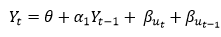
The equation above follows the first order of autoregressive process or AR(1) and the value of p is 1. Hence the value of Yt in the period ‘t’ depends upon its previous year value and a random term.
Moving Average (MA) Process :- When the value of Yt of order q in a time series data depends on the weighted sum of current and the q recent errors i.e. a linear combination of error terms then it is called a moving average process which can be written as :-
yt = observation which we need to find out
α= constant term
βut-q= error over the period q .
ARMA (Autoregressive Moving Average) Process :-
The above equation shows that value of Y in time period ‘t’ can be derived by taking into consideration the order of lag p which in the above case is 1 i.e. previous year’s observation and the weighted average of the error term over a period of time q which in case of the above equation is 1.
How to decide the value of p and q?
Two of the most important methods to obtain the best possible values of p and q are ACF and PACF plots.
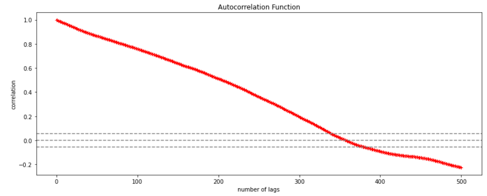
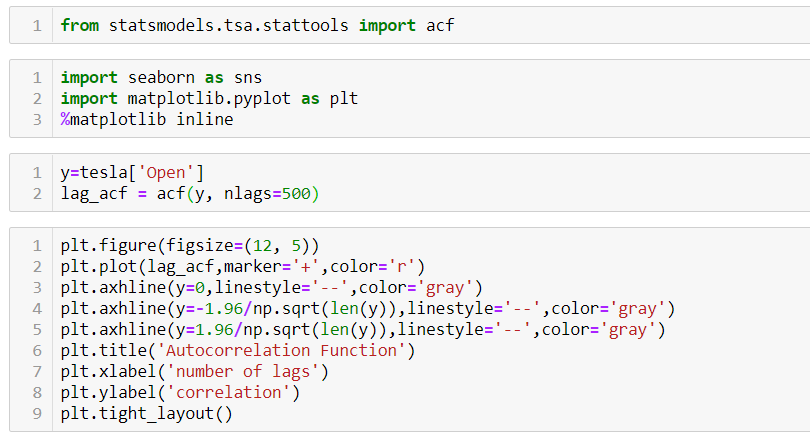
ACF (Auto-correlation function) :- This function calculates the auto-correlation of the complete data on the basis of lagged values which when plotted helps us choose the value of q that is to be considered to find the value of Yt. In simple words how many years residual can help us predict the value of Yt can obtained with the help of ACF, if the value of correlation is above a certain point then that amount of lagged values can be used to predict Yt.
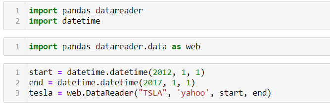
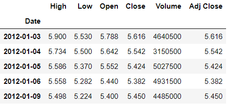
Using the stock price of tesla between the years 2012 and 2017 we can use the .acf() method in python to obtain the value of p.
.DataReader() method is used to extract the data from web.
The above graph shows that beyond the lag 350 the correlation moved towards 0 and then negative.
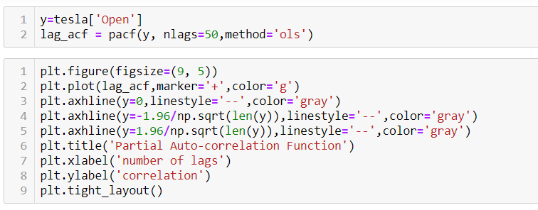
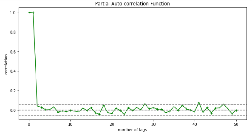
PACF (Partial auto-correlation function) :- Pacf helps find the direct effect of the past lag by removing the residual effect of the lags in between. Pacf helps in obtaining the value of AR where as acf helps in obtaining the value of MA i.e. q. Both the methods together can be use find the optimum value of p and q in a time series data set.
Lets check out how to apply pacf in python.
As you can see in the above graph after the second lag the line moved within the confidence band therefore the value of p will be 2.
So, with that we come to the end of the discussion on the ARMA Model. Hopefully it helped you understand the topic, for more information you can also watch the video tutorial attached down this blog. The blog is designed and prepared by Niharika Rai, Analytics Consultant, DexLab AnalyticsDexLab Analytics offers machine learning courses in Gurgaon. To keep on learning more, follow DexLab Analytics blog.
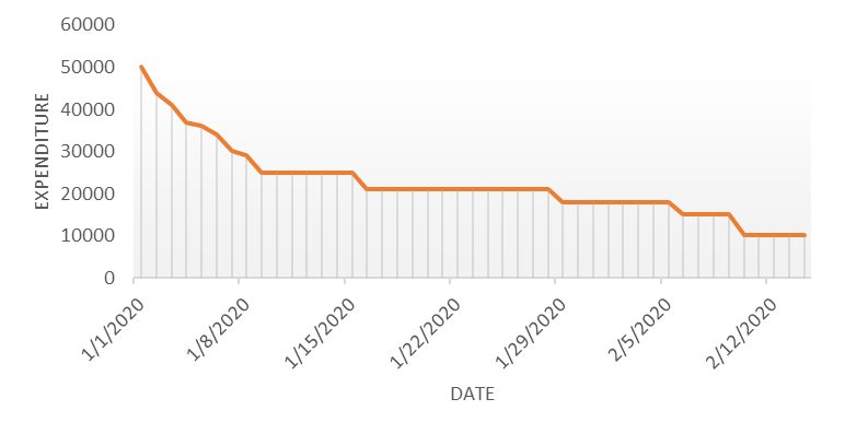
Autocorrelation is a special case of correlation. It refers to the relationship between successive values of the same variables .For example if an individual with a consumption pattern:-
spends too much in period 1 then he will try to compensate that in period 2 by spending less than usual. This would mean that Ut is correlated with Ut+1 . If it is plotted the graph will appear as follows :
Positive Autocorrelation : When the previous year’s error effects the current year’s error in such a way that when a graph is plotted the line moves in the upward direction or when the error of the time t-1 carries over into a positive error in the following period it is called a positive autocorrelation. Negative Autocorrelation : When the previous year’s error effects the current year’s error in such a way that when a graph is plotted the line moves in the downward direction or when the error of the time t-1 carries over into a negative error in the following period it is called a negative autocorrelation.
Now there are two ways of detecting the presence of autocorrelation By plotting a scatter plot of the estimated residual (ei) against one another i.e. present value of residuals are plotted against its own past value.
If most of the points fall in the 1st and the 3rd quadrants , autocorrelation will be positive since the products are positive.
If most of the points fall in the 2nd and 4th quadrant , the autocorrelation will be negative, because the products are negative. By plotting ei against time : The successive values of ei are plotted against time would indicate the possible presence of autocorrelation .If e’s in successive time show a regular time pattern, then there is autocorrelation in the function. The autocorrelation is said to be negative if successive values of ei changes sign frequently. First Order of Autocorrelation (AR-1) When t-1 time period’s error affects the error of time period t (current time period), then it is called first order of autocorrelation. AR-1 coefficient p takes values between +1 and -1 The size of this coefficient p determines the strength of autocorrelation. A positive value of p indicates a positive autocorrelation. A negative value of p indicates a negative autocorrelation In case if p = 0, then this indicates there is no autocorrelation. To explain the error term in any particular period t, we use the following formula:-
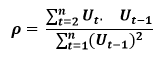
Where Vt= a random term which fulfills all the usual assumptions of OLS How to find the value of p?
One can estimate the value of ρ by applying the following formula :-
Data Smoothing is done to better understand the hidden patterns in the data. In the non- stationary processes, it is very hard to forecast the data as the variance over a period of time changes, therefore data smoothing techniques are used to smooth out the irregular roughness to see a clearer signal.
In this segment we will be discussing two of the most important data smoothing techniques :-
Moving average smoothing
Exponential smoothing
Moving average smoothing
Moving average is a technique where subsets of original data are created and then average of each subset is taken to smooth out the data and find the value in between each subset which better helps to see the trend over a period of time.
Lets take an example to better understand the problem.
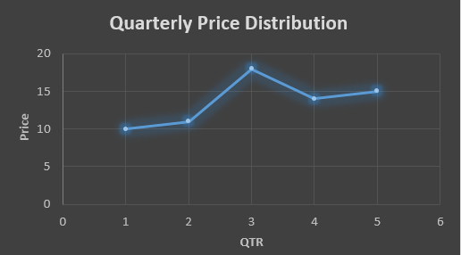
Suppose that we have a data of price observed over a period of time and it is a non-stationary data so that the tend is hard to recognize.
QTR (quarter)
Price
1
10
2
11
3
18
4
14
5
15
6
?
In the above data we don’t know the value of the 6th quarter.
….fig (1)
The plot above shows that there is no trend the data is following so to better understand the pattern we calculate the moving average over three quarter at a time so that we get in between values as well as we get the missing value of the 6th quarter.
To find the missing value of 6th quarter we will use previous three quarter’s data i.e.
MAS = = 15.7
QTR (quarter)
Price
1
10
2
11
3
18
4
14
5
15
6
15.7
MAS = = 13
MAS = = 14.33
QTR (quarter)
Price
MAS (Price)
1
10
10
2
11
11
3
18
18
4
14
13
5
15
14.33
6
15.7
15.7
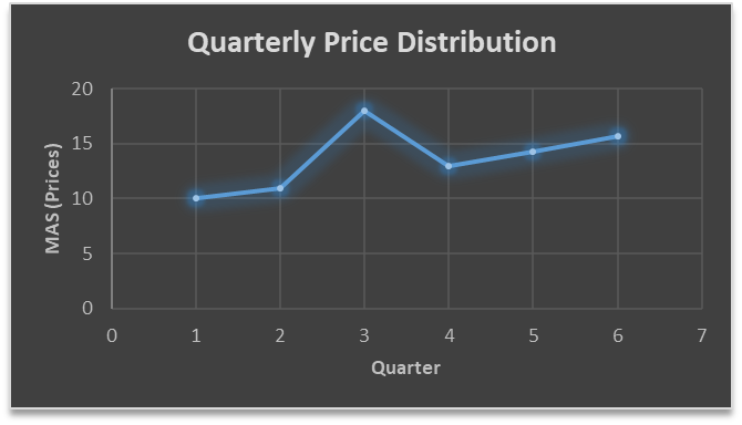
….. fig (2)
In the above graph we can see that after 3rd quarter there is an upward sloping trend in the data.
Exponential Data Smoothing
In this method a larger weight ( ) which lies between 0 & 1 is given to the most recent observations and as the observation grows more distant the weight decreases exponentially.
The weights are decided on the basis how the data is, in case the data has low movement then we will choose the value of closer to 0 and in case the data has a lot more randomness then in that case we would like to choose the value of closer to 1.
EMA= Ft= Ft-1 + (At-1 – Ft-1)
Now lets see a practical example.
For this example we will be taking = 0.5
Taking the same data……
QTR (quarter)
Price
(At)
EMS Price(Ft)
1
10
10
2
11
?
3
18
?
4
14
?
5
15
?
6
?
?
To find the value of yellow cell we need to find out the value of all the blue cells and since we do not have the initial value of F1 we will use the value of A1. Now lets do the calculation:-
F2=10+0.5(10 – 10) = 10
F3=10+0.5(11 – 10) = 10.5
F4=10.5+0.5(18 – 10.5) = 14.25
F5=14.25+0.5(14 – 14.25) = 14.13
F6=14.13+0.5(15 – 14.13)= 14.56
QTR (quarter)
Price
(At)
EMS Price(Ft)
1
10
10
2
11
10
3
18
10.5
4
14
14.25
5
15
14.13
6
14.56
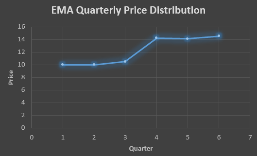
14.56
In the above graph we see that there is a trend now where the data is moving in the upward direction.
So, with that we come to the end of the discussion on the Data smoothing method. Hopefully it helped you understand the topic, for more information you can also watch the video tutorial attached down this blog. The blog is designed and prepared by Niharika Rai, Analytics Consultant, DexLab AnalyticsDexLab Analytics offers machine learning courses in Gurgaon. To keep on learning more, follow DexLab Analytics blog.
A time series is a sequence of numerical data in which each item is associated with a particular instant in time. Many sets of data appear as time series: a monthly sequence of the quantity of goods shipped from a factory, a weekly series of the number of road accidents, daily rainfall amounts, hourly observations made on the yield of a chemical process, and so on. Examples of time series abound in such fields as economics, business, engineering, the natural sciences (especially geophysics and meteorology), and the social sciences.
Univariate time series analysis- When we have a single sequence of data observed over time then it is called univariate time series analysis.
Multivariate time series analysis – When we have several sets of data for the same sequence of time periods to observe then it is called multivariate time series analysis.
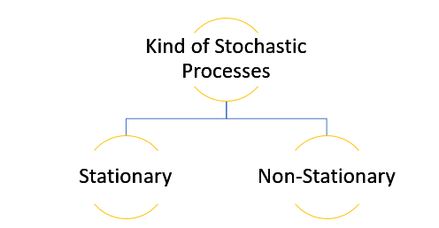
The data used in time series analysis is a random variable (Yt) where t is denoted as time and such a collection of random variables ordered in time is called random or stochastic process.
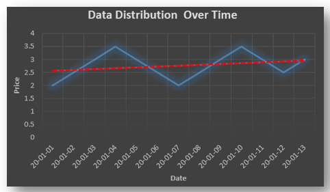
Stationary: A time series is said to be stationary when all the moments of its probability distribution i.e. mean, variance , covariance etc. are invariant over time. It becomes quite easy forecast data in this kind of situation as the hidden patterns are recognizable which make predictions easy.
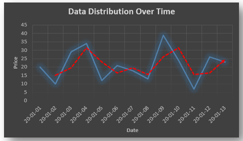
Non-stationary: A non-stationary time series will have a time varying mean or time varying variance or both, which makes it impossible to generalize the time series over other time periods.
Non stationary processes can further be explained with the help of a term called Random walk models. This term or theory usually is used in stock market which assumes that stock prices are independent of each other over time. Now there are two types of random walks: Random walk with drift : When the observation that is to be predicted at a time ‘t’ is equal to last period’s value plus a constant or a drift (α) and the residual term (ε). It can be written as Yt= α + Yt-1 + εt The equation shows that Yt drifts upwards or downwards depending upon α being positive or negative and the mean and the variance also increases over time. Random walk without drift: The random walk without a drift model observes that the values to be predicted at time ‘t’ is equal to last past period’s value plus a random shock. Yt= Yt-1 + εt Consider that the effect in one unit shock then the process started at some time 0 with a value of Y0 When t=1 Y1= Y0 + ε1 When t=2 Y2= Y1+ ε2= Y0 + ε1+ ε2 In general, Yt= Y0+∑ εt In this case as t increases the variance increases indefinitely whereas the mean value of Y is equal to its initial or starting value. Therefore the random walk model without drift is a non-stationary process.
So, with that we come to the end of the discussion on the Time Series. Hopefully it helped you understand time Series, for more information you can also watch the video tutorial attached down this blog. DexLab Analytics offers machine learning courses in delhi. To keep on learning more, follow DexLab Analytics blog.
Artificial Intelligence, or, its more popular acronym AI is no longer a term to be read about in a sci-fi book, it is a reality that is reshaping the world by introducing us to virtual assistants, helping us be more secure by enabling us with futuristic measures. The evolution of AI has been pretty consistent and as we are busy navigating through a pandemic-ridden path towards the future, adapting to the “new normal”, and becoming increasingly reliant on technology, AI assumes a greater significance.
The AI applications which are already being implemented has resulted in a big shift, causing an apprehension that the adoption of AI technology on a larger scale would eventually lead to job cuts, whereas in reality, it would lead to the creation of new jobs across industries. Adoption of AI technology would push the demand for a workforce that is highly skilled, enrolling in an artificial intelligence course in delhi could be a timely decision.
Now that we are about to reach the end of 2020, let us take a look at the possible impacts of AI in the future.
AI will create more jobs
Yes, contrary to the popular apprehension AI would end up creating jobs in the future. However, the adoption of AI to automate tasks means yes, there would be a shift, and a job that does not need special skills will be handled by AI powered tools. Jobs that could be done without error, completed faster, with a higher level of efficiency, in short better than humans could be performed by robots. However, with that being said there would be more specialized job roles, remember AI technology is about the simulation of human intelligence, it is not the intelligence, so there would be humans in charge of carrying out the AI operated areas to monitor the work. Not just that but for developing smarter AI application and implementation there should be a skilled workforce ready, a report by World Economic Forum is indicative of that. From design to maintenance, AI specialists would be in high demand especially the developers. The fourth industrial revolution is here, industries are gearing up to build AI infrastructure, it is time to smell the coffee as by the end of 2022 there will be millions of AI jobs waiting for the right candidates.
Dangerous jobs will be handled by robots
In the future, hazardous works will be handled by robots. Now the robots are already being employed to handle heavy lifting tasks, along with handling the mundane ones that require only repetition and manual labor. Along with automating these tasks, the robot workforce can also handle the situation where human workers might sustain grave injuries. If you have been aware and interested then you already heard about the “SmokeBot”. In the future, it might be the robots who will enter the flaming buildings for assessment before their human counterparts can start their task. Manufacturing plants that deal with toxic elements need robot workers, as humans run a bigger risk when they are exposed to such chemicals. Furthermore, the nuclear plants might have a robot crew that could efficiently handle such tasks. Other areas like pipeline exploration, bomb defusing, conducting rescue operations in hostile terrain should be handled by AI robots.
Smarter healthcare facilities
AI implementation which has already begun would continue to transform the healthcare services. With AI being in place CT scan and MRI images could be more precise pointing out even minuscule changes that earlier went undetected. Drug development could also be another area that would see vast improvement and in a post-pandemic world, people would need to be better prepared to fight against such viruses. Real-time detection could prevent many health issues going severe and keeping a track of the health records preventive measures could be taken. One of the most crucial changes that could be revolutionary, is the personalized medication which could only be driven by AI technology. This would completely change the way healthcare functions. Now that we are seeing chat bots for handling sales queries, the future healthcare landscape might be ruled by virtual assistants specifically developed for offering assistance to the patients. There are going to be revolutionary changes in this field in the future, thereby pushing the demand for professionals skilled in deep learning for computer vision with python.
Smarter finance
We are already living in an age where we have robo advisors, this is just the beginning and the growing AI implementation would enable an even smarter analytics system that would minimize the credit risk and would allow banks and other financial institutes to minimize the risk of fraud. Smarter asset management, enhanced customer support are going to be the core features. Smarter ML algorithms would detect any and every oddity in behavior or in transactions and would help prevent any kind of fraud from happening. With analytics being in place it would be easier to predict the future trends and thereby being more efficient in servicing the customers. The introduction of personalized services is going to be another key feature to look out for.
Retail space gets a boost
The retailers are now aiming to implement AI applications to offer smart shopping solutions to the future buyers. Along with coming up with personalized shopping suggestions for the customers and showing them suggestions based on their shopping pattern, the retailers would also be using the AI to predict the future trends and work accordingly. Not just that but they can easily maintain the supply and demand balance with the help of AI solutions and stock up items that are going to be in demand instead of items that would not be trendy. The smarter assistants would ensure that the customer queries are being handled and they could also be helping them with shopping by providing suggestions and information. From smart marketing to smarter delivery, the future of retail would be dominated by AI as the investment in this space is gradually going up.
The future is definitely going to be impacted by the AI technology in more ways than one. So, be future ready and get yourself upskilled as it is the need of the hour, stay updated and develop the skill to move towards the AI future with confidence.
This is a tutorial where we teach you to do image recognition using LSTM. To get to the core you have to understand that how a convolutional neural network perceives the data. In this tutorial the data we have is four-dimensional data, so, you need to convert the dataset accordingly. You can find the tutorial video attached to this blog.
Now suppose there is an image 28 by 28 pixel, if the image is black and white then there would be only one channel. So how will you put the data in CNN, it will be like the number of samples, then followed by the number of rows of the data, then the number of columns, then channels. These are the four values that need to be provided in the input layer, at the very beginning. Now, these values must be converted according to the LSTM. Now the LSTM wants the STF, like the number of samples, time steps like how many time steps back you want to go for making further prediction because LSTM is a sequence generator and the number of features. So, we will be converting the image that is the number of sample 28 by 28 one pixel into one sample of 28 by 28, that’s the only job you have to do and all you need to accomplish this is to prepare the data accordingly.
There will be no mysteries here, in fact, it is a normal neural network LSTM, that anybody can run in a most simple form, and in this tutorial, it is also run in the most simple form there is no complexity involved and only a few epochs will be run.
You can find the code sheet you need for this at
Also follow this video that explains the process step by step, so that you can easily grasp how LSTM can be used for the purpose of image recognition. To access more informative tutorial sessions like this follow the DexLab Analytics blog.
AI is a dynamic field that is constantly evolving thanks to the continuous stream of research work being conducted. The field is being reshaped by emerging trends. In order to keep pace with this fast-moving technology, especially if you are pursuing Data Science training you should learn about the latest trends that are going to dominate this field.
Digital Data Forgetting
It is a curious trend to watch out for as instead of learning data, unlearning would take precedence. In machine learning data is fed to the system based on which it makes predictive analysis. However, thanks to the growing channels and activities the amount of data generated is increasing, and a significant portion of which might not even be required and which only contribute to creating noise.
Although it is possible to store the data utilizing cloud-based systems, the price an organization will have to bear for unnecessary data, does not justify the decision. Furthermore, it might also raise privacy risks in the future. The efficient handling of this data lineage issue requires systems that will forget unnecessary data so that it can proceed with what is important.
NLP
Now that chatbots are being put to use to provide better customer support, the significance of NLP or, natural language processing is only going to increase. NLP is all about analyzing and processing speech patterns. There is now a shift towards developing language models around the concepts of pre-training and fine-tuning and further research work is being conducted to make these systems even more efficient, however, the focus on transfer learning might lessen considering the financial and operational complications involved in the process.
Reinforcement Learning
This is another trend to look out for, reinforcement learning is where a model or system learning involves a preset goal and is met with reward or, punishment depending upon the outcome. This particular trend might push AI to a whole new level. In RL, the learning activity is somewhat random and the system has to rely on the experience it has gained and continues to learn by repeating what it has learned, and as it starts recognizing rewards it continues working towards it until the learning takes a logical turn. Research works are being conducted to make this process more sophisticated.
Automated Machine Learning
If you are aware of Google AutoML, then you already have an inkling of what AutoML is. It basically focuses on the end-to-end process and automates it. It applies a number of techniques including RL, to reach a higher level of accuracy. It works on raw data and processes it to suggest a solution that is most appropriate. It basically is a lifesaver for those who are not familiar with ML. However, there are programs available that enable professionals pursue Machine Learning Using Python who are looking to gain expertise in this field.
Internet of Things
IOT devices are a rage and they are able to collect a huge amount of user data that needs to be processed to gather valuable information. However, there could be certain challenges involved in the data collection process which lead to error. The application of ML in this particular field can not only lend more efficiency to the way IOT operates but it can also process a large amount of data to offer actionable insight. The information filtered this way could help develop efficient models for businesses and various other sectors. The merger of IOT and ML is definitely a trend that is definitely going to be revolutionary.
AI technology is getting more sophisticated with emerging trends. The manifold application of AI is opening up new career avenues. Enrolling in a premier artificial intelligence training institute in Gurgaon, would be a good career move for anybody looking forward to having a career in this domain.
The world has seen a transformation in its economic activities since the coronavirus pandemic broke out. Economies have come to a grinding halt and manufacturing has dipped. Now what nations need is resilience and strength to carry on production in all sectors. What they are most depending on is the power of Artificial Intelligence to enhance the manufacturing process and help save money and drive down costs.
Here are some examples of how AI is powering the manufacturing sector in 2020.
AI is being used to transform machinery maintenance and quality in manufacturing operations today, according to Capgemini.
Caterpillar’s Marine Division is using machine learning to analyze data on how often its shipping equipment should be cleaned helping it save thousands of dollars.
The BMW Group is using AI to study manufacturing component images in and spot deviations from the standard production procedure in real-time.
In fact, a study shows that in the four earlier global economic downturns companies using AI were actually successful in increasing both sales and profit margins. Companies are all striving to utilize human experience, insights and AI techniques to give manufacturing a fillip in these times of a crisis.
Manufacturing using AI in real-time
Real-time monitoring of the manufacturing process is advantageous because it translates to sorting out production bottlenecks, tracking scrap rates and meeting customer deadlines among other things. The huge cache of data used can be utilized to build machine learning models.
Supervised and unsupervised machine learning algorithms can study multiple production shifts’ real-time data within seconds and predict processes, products, and workflow patterns that were not known before. A report suggests 29% of AI implementations in manufacturing are for maintaining machinery and production assets.
Detecting Outages
It was found that the most popular use of AI in manufacturing is predicting when equipment are likely to fail and suggesting optimal times to conduct maintenance. Companies like General Motors analyze images of its robots from cameras mounted above to spot anomalies and possible failures in the production line and thus preempt outages.
Optimizing Design
General Motors uses AI algorithms to give and produce optimized product design. General Motors can achieve the goal of rapid prototyping with the help of AI and ML algorithms. Designers provide definitions of the functional needs, raw materials, manufacturing methods and other constraints and the company along with AutoDesk has customized Dreamcatcher to optimize for weight and other vital criterion. In this way, AI comes together with human endeavor to produce a-class product designs that cost lesser.
Inconsistencies
Nokia has begun using a video application that takes the help of machine learning to alert an assembly operator if there are inconsistencies in the production process in one of its factories in Oulu, Finland. It alerts a machine operator about inconsistencies in the production of electronic items and this helps preempt poor production process and helps the company save on a lot of money and capital.
There are many other production processes AI is helping revolutionize. Only time will tell how much of AI will power the manufacturing sector. But this technological advancement is surely making an impact on economies worldwide. Meanwhile, for more details, do peruse the DexLab Analytics website. DexLab Analytics is a premiere machine learning institute in Gurgaon.