As we continue our discussion on statistical inference, we move on to the estimation theory. Here you will learn about the concept of estimation, along with different elements and methods of estimation. You can check part-II here.
Content:
- Introduction
- Element of Estimation (Parameter, Statistic, Relation between Statistic and Parameter
- What is Estimation (Point estimation, Interval estimation)
- Characteristics of Estimation (Unbiasedness)
- Characteristics of Estimation (Sufficiency, Efficiency, Consistency)
- Method of Estimation (MLE, MLS)
- Method of Estimation (MMV, MM)
- Conclusion
Introduction
The estimation is the process of providing numerical values of the unknown parameter to the population. There are mainly two types of estimation process Point estimation and Interval estimation and confidence interval is the part of the interval estimation. We will also discuss about the elements of the estimation like parameter, statistic and estimator.
The characteristics of estimators are – (i) Unbiasedness – This is desirable property of a good estimator. (ii) Consistency – An estimator is said to be consistent if increasing the sample size produces an estimate with smaller standard error. (iii) Efficiency – An estimator should be an efficient estimator. (iv) Sufficiency – An estimator is said to be sufficient for a parameter, if it contains all the information in the sample regarding the parameter.
The methods of estimation are– (i) Method of maximum likelihood, (ii) Method of least square, (iii) Method of minimum variance, (iv) Method of moments.
Element For Estimation
Parameter
Parameter is an unknown numerical factor of the population. The primary interest of any survey lies in knowing the values of different measures of the population distribution of a variable of interest. The measures of population distribution involves its mean, standard deviation etc. which is calculated on the basis of the population values of the variable. In other words, the parameter is a functional form of all the population unit.
Statistic
Any statistical measure calculated on the basis of sample observations is called Statistic. Like sample mean, sample standard deviation, etc. Sample statistic are always known to us.
Estimator An estimator is a measure computed on the basis of sample values. It is a functional from of all sample observe prorating a representative value of the collected sample. Relation Between Parameter And Statistic
Parameter is a fixed measure describing the whole population (population being a group of people, things, animals, phenomena that share common characteristics.) A statistic is a characteristic of a sample, a portion of the target population. A parameter is fixed, unknown numerical value, while the statistic is a known number and a variable which depends on the portion of the population. Sample statistic and population parameters have different statistical notations: In population parameter, population proportion is represented by P, mean is represented by µ (Greek letter mu), σ2 represents variance, N represents population size, σ (Greek letter sigma) represents standard deviation, σx̄ represents Standard error of mean, σ/µ represents Coefficient of variation, (X-µ)/σ represents standardized variate (z), and σp represents standard error of proportion.
In sample statistics, mean is represented by x̄(x-bar), sample proportion is represented by p̂(p-hat), s represents standard deviation, s2 represents variance, sample size is represented by n, sx̄ represents Standard error of mean, sp represents standard error of proportion, s/(x̄) represents Coefficient of variation, and (x-x)/s ̄ represents standardized variate (z).
What Is Estimation?
Estimation refers to the process by which one makes an idea about a population, based on information obtained from a sample.
Suppose we have a random sample 𝑥1, 𝑥2, … , 𝑥𝑛 on a variable x, whose distribution in the population involves an unknown parameter 𝜃. It is required to find an estimate of 𝜃 on the basis of sample values. The estimation is done in two different ways: (i) Point Estimation, and (ii) Interval Estimation.
In point estimation, the estimated value is given by a single quantity, which is a function of sample observations. This function is called the ‘estimator’ of the parameter, and the value of the estimator in a particular sample is called an ‘estimate’.
Interval estimation, an interval within which the parameter is expected to lie in given by using two quantities based on sample values. This is known as Confidence interval, and the two quantities which are used to specify the interval, are known as Confidence Limits.
Point Estimation
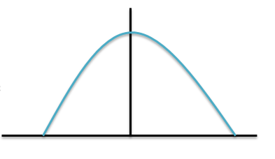
Many functions of sample observations may be proposed as estimators of the same parameter. For example, either the mean or median or mode of the sample values may be used to estimate the parameter 𝜇 of the normal distribution with probability density function
 Which we shall in future refer to as 𝑁(𝜇, 𝜎 2 ).
Interval Estimation
In statistical analysis it is not always possible to find out an exact point estimate to form an idea about the population parameters. An approximately true picture can be formed if the sample estimations satisfy some important property such as unbiasedness consistency, sufficiency, efficiency & so on. So, a more general concept of estimation would be to find out an interval based on sample values which is expected to include the unknown parameter with a specified probability. This is known as the theory of interval estimator.
Confidence Interval
Let 𝑥1, 𝑥2,… , 𝑥𝑛 be a random sample from a population involve an unknown parameter 𝜃. Our job is to find out two functions 𝑡1 & 𝑡2 of the sample values. Such that the probability of 𝜃 being included in the random interval 𝑡1,𝑡2 has a given value say 1 − 𝛼 . So,
Here the interval [𝑡1,𝑡2] is called a 100 × ( ) 1 − 𝛼 % confidence interval for the parameter 𝜃. The quantities 𝑡1 & 𝑡2 which serve as the lower & upper limits of the interval are known as confidence limits. 1 − 𝛼 is called the confidence coefficient. The is a sort of measures of the trust or confidence that one may place in the interval for actually including 𝜃.
Characteristics of Estimation
Unbiasedness
A statistic t is said to be an Unbiased Estimator of parameter 𝜃, if the expected value of t is 𝜃. 𝐸 𝑡 = 𝜃 Otherwise, the estimator is said to be ‘biased’. The bias of a statistic in estimating 𝜃 is given as 𝐵𝑖𝑎𝑠 = 𝐸 𝑡 − 𝜃 Let 𝑥1, 𝑥2,… , 𝑥𝑛 be a random sample drawn from a population with mean 𝜇 and variance 𝜎 2 . Then Sample mean
 Sample variance
 The sample mean 𝑥ҧis an unbiased estimator of the population mean 𝜇; because 𝐸 𝑥ҧ = 𝜇 The sample variance 𝑆 2 is a biased estimator of the population variance 𝜎 2 ; because
An unbiased estimator of the population variance 𝜎 2 is given by ![]()
Because
The distinction between 𝑆 2 and 𝑠 2 in which only he denominators are different. 𝑆 2 is the variance of the sample observations, but 𝑠 2 is the ‘unbiased estimator’ of the variance (𝜎 2 ) in the population.
Example:
Characteristics of Estimation (Sufficiency, Efficiency, Consistency)
Consistency
A desirable property of good estimator is that its accuracy should increase when the sample becomes larger. That is, the estimator is expected to come closer to the parameter as the size of the sample increases.
A statistic 𝑡𝑛 computed from a sample of n observations is said to be a Consistent Estimator of a parameter 𝜃, if it converges in probability to 𝜃 as n tends to infinity. This means that the larger the sample size (n), the less is the chance that the difference between 𝑡𝑛 and 𝜃 will exceed any fixed value. In symbols, given any arbitrary small positive quantity 𝜖, ![]() 𝜇 , then the statistic 𝑡𝑛 will be a ‘consistent estimator’ of 𝜃. Consistency is a limiting property. Moreover, several consistent estimators may exist for the same parameter. For example, in sampling from a normal population 𝑁 𝜇, 𝜎 2 , both the sample mean and sample median are consistent estimators of 𝜇.
𝜇 , then the statistic 𝑡𝑛 will be a ‘consistent estimator’ of 𝜃. Consistency is a limiting property. Moreover, several consistent estimators may exist for the same parameter. For example, in sampling from a normal population 𝑁 𝜇, 𝜎 2 , both the sample mean and sample median are consistent estimators of 𝜇.
Efficiency
If we confine ourselves to unbiased estimates, there will, in general, exist more than one consistent estimator of a parameter. For example, in sampling from a normal population 𝑁 𝜇, 𝜎 2 , when 𝜎 2 is known, sample mean 𝑥ҧis an unbiased and consistent estimator of 𝜇. From symmetry it follows immediately the sample median (Md) is an unbiased estimate of 𝜇. Which is same as the population median. Also for large n,
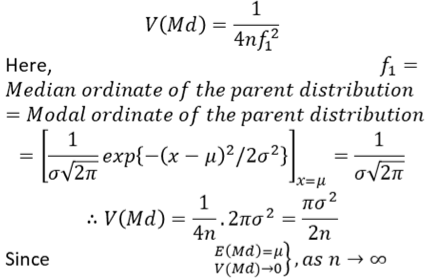 Median is also an unbiased and consistent estimator of 𝜇.
Thus, there is necessity of some further criterion which will enable us to choose between the estimators with the common property of consistency.
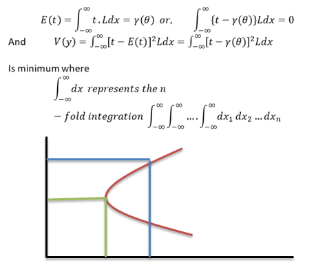
Such a criterion which is based on the variance of the sampling distribution of estimators is usually known as Efficiency.
Sufficiency
A statistic is said to be a ‘sufficient estimator’ of a parameter 𝜃, if it contains all information in the sample about 𝜃. If a statistic t exists such that the joint distribution of the sample is expressible as the product of two factors, one of which is the sampling distribution of t and contains 𝜃, but the other factor is independent of 𝜃, then t will be a sufficient estimator of 𝜃.
Thus if 𝑥1, 𝑥2,… , 𝑥𝑛 is a random sample from a population whose probability mass function or probability density function is 𝑓 𝑥, 𝜃 , and t is a sufficient estimator of 𝜃 then we can write
![]() Where g(t, 𝜃) is the sampling distribution of t and contains 𝜃, but ℎ (𝑥1, 𝑥2,… , 𝑥𝑛) is independent of 𝜃.
Where g(t, 𝜃) is the sampling distribution of t and contains 𝜃, but ℎ (𝑥1, 𝑥2,… , 𝑥𝑛) is independent of 𝜃.
Since the parameter 𝜃 is occurring in the joint distribution of all the sample observations can be contained in the distribution of the statistic t, it is said that t alone can provide all ‘information’ about 𝜃 and is therefore “sufficient” for 𝜃.
Sufficient estimators are the most desirable kind of estimators, but unfortunately they exist in only relatively few cases. If a sufficient estimator exists, it can be found by the method of maximum likelihood.
In random sampling from a Normal population 𝑁 (𝜇, 𝜎 2) , the sample mean 𝑥ҧis a sufficient estimator of 𝜇.
Methods of Estimation (MLE, MLS)
Method of Maximum Likelihood
This is a convenient method for finding an estimator which satisfies most of the criteria discussed earlier. Let 𝑥1, 𝑥2,… , 𝑥𝑛 be a random sample from a population with p.m.f (for discrete case) or p.d.f. (for continuous case) 𝑓 𝑥, 𝜃 , where 𝜃 is the parameter. Then the joint distribution of the sample observations
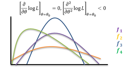
![]() is called the Likelihood Function of the sample. The Method of Maximum Likelihood consists in choosing as an estimator of 𝜃 that statistic, which when substituted for 𝜃, maximizes the likelihood function L. such a statistic is called a maximum likelihood estimator (m.l.e.). We shall denote the m.l.e. of 𝜃 by the symbol 𝜃0. Since log 𝐿 is maximum when L is maximum, in practice the m.l.e. of 𝜃 is obtained by maximizing log 𝐿 . This is achieved by differentiating log 𝐿 partially with respect to 𝜃, and using the two relations
is called the Likelihood Function of the sample. The Method of Maximum Likelihood consists in choosing as an estimator of 𝜃 that statistic, which when substituted for 𝜃, maximizes the likelihood function L. such a statistic is called a maximum likelihood estimator (m.l.e.). We shall denote the m.l.e. of 𝜃 by the symbol 𝜃0. Since log 𝐿 is maximum when L is maximum, in practice the m.l.e. of 𝜃 is obtained by maximizing log 𝐿 . This is achieved by differentiating log 𝐿 partially with respect to 𝜃, and using the two relations
The m.l.e. is not necessarily unbiased. But when the m.l.e. is biased, by a slight modification, it can be converted into an unbiased estimator. The m.l.e. tends to be distributed normally for large samples. The m.l.e. is invariant under functional transformations. If T is an m.l.e. of 𝜃, and 𝑔(𝜃) is a function of 𝜃, then g(T) is the m.l.e. of 𝑔(𝜃) .
Method Of Least Square
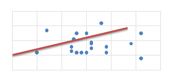
Method of Least Squares is a device for finding the equation of a specified type of curve, which best fits a given set of observations. The principal of least squares is used to fit a curve of the form:
𝑦𝑖 = 𝑓 𝑥𝑖 be a function where 𝑥𝑖 is an explanatory variable. & 𝑦𝑖 is the dependent variable. Let us assume a linear relationship between the dependent & independent variable. So,
𝑌𝑖 = 𝛼 + 𝛽𝑥𝑖 + 𝑒𝑖 ; 𝛼 = 𝑖𝑛𝑡𝑒𝑟𝑐𝑒𝑝𝑡 𝑓𝑜𝑟𝑚 𝛽 = 𝑅𝑒𝑠𝑝𝑜𝑛𝑠𝑖𝑣𝑒𝑛𝑒𝑠𝑠 𝑜𝑓 𝑌𝑖 𝑒𝑖 = 𝐸𝑟𝑟𝑜𝑟 𝑓𝑜𝑟𝑚
The objective of the researcher is to minimize σ𝑙𝑖 2, σ 𝑒𝑖 is not minimized because σ 𝑒𝑖 = 0 but actual error of individual observation can remain
The method of least squares can be used to fit other types of curves, e.g. parabola, exponential curve, etc. method of least squares is applied to find regression lines and also in the determination of trend in time series.
Methods of Estimation (MMV, MM)
Method of Minimum Variance
Minimum Variance Unbiased Estimates, the estimates 𝑖 𝑇 𝑖𝑠 𝑢𝑛𝑏𝑖𝑎𝑠𝑒𝑑 𝑓𝑜𝑟 𝛾 𝜃 , 𝑓𝑜𝑟 𝑎𝑙𝑙 𝜃𝜖𝜗 are unbiased and [(ii) It has smallest variance among the class of all unbiased estimators of 𝛾(𝜃), then T is called the minimum variance unbiased estimator (MVUE) of 𝛾(𝜃)] have minimum variance.
If 𝐿 = ς𝑖=1 𝑛 𝑓 𝑥𝑖 , 𝜃 , is the likelihood function of a random sample of n observations 𝑥1, 𝑥2, … , 𝑥𝑛 from a population with probability function 𝑓(𝑥, 𝜃), then the problem is to find a statistics 𝑡 = 𝑡(𝑥1, 𝑥2,… , 𝑥𝑛), such that
This method was discovered and studied in detail by Karl Pearson. Let 𝑓 𝑥; 𝜃1, 𝜃2, … , 𝜃𝑘 be the density function of the parent population with k parameters 𝜃1, 𝜃2,… , 𝜃𝑘. If 𝜇𝑟 ′ denoted the rth moment about origin, then
 Let 𝑥𝑖 , 𝑖 = 1,2, … , 𝑛 be a random sample of size n from the given population. The method of moments consists in solving the k-equations for 𝜃1, 𝜃2,… , 𝜃𝑘 in terms of 𝜇1 ′ , 𝜇2 ′ ,… , 𝜇𝑘 ′ and then replacing these moments 𝜇𝑟 ′ ; 𝑟 = 1,2,… , 𝑘 by the sample moments,
Where 𝑚𝑖 ′ is the ith moment about origin in the sample.
Then by the method of moments 𝜃1, 𝜃2,… , 𝜃𝑘 are the required estimator of 𝜃1, 𝜃2,… . , 𝜃𝑘 respectively.
Conclusion
Estimation theory is a branch of statistics and signal processing that deals with estimating the values of parameters based on measured/empirical data that has a random component. The parameters describe an unknown numerical factor of the population. The primary interest of any survey lies in knowing the values of different measures of the population distribution of a variable of interest. The measures of population distribution involves its mean, standard deviation etc. which is calculated on the basis of the population values of the variable. The estimation theory has its own characteristics like the data should be unbiased, a good estimator is that its accuracy should increase when the sample size becomes larger, The sample mean and sample median should be consistent estimators of parameter mean, The estimator is expected to come closer to the parameter as the size of the sample increases. Two consistent estimators for the same parameter, the statistic with the smaller sampling variance is said to be more efficient, so, efficiency is another characteristic of the estimation. The estimator should be sufficient estimator of a parameter theta.
The estimation theory follows some methods by this method and with the characteristics we can properly estimate from the data. The methods we already discussed that maximum likelihood method, least square method, minimum variance method & method of moments.
In real life, estimation is part of our everyday experience. When you’re shopping in the grocery store and trying to stay within a budget, for example, you estimate the cost of the items you put in your cart to keep a running total in your head. When you’re purchasing tickets for a group of people or splitting the cost of dinner between 8 friends, we estimate for ease. In many other field we can use the estimation theory specially for statistical analysis.
If you found this blog helpful then, then keep on exploring DexLab Analytics blog to pursue more informative posts on diverse topics such as python for data analysis. Also, check out part-I AND part- II of the series to keep pace.
.
Business analysis training, business analytics, business analytics certification, business analytics course in delhi
