Internet of Things or IOT devices are a rage now, as these devices staying connected to the internet can procure data and exchange the same using the sensors embedded in those. Now the data which is being generated in copious amount needs to be processed and in comes IoT Analytics. This platform basically is concerned with analyzing the large amount of data generated by the devices. The interconnectivity of devices is helping different sectors be in sync with the world, and the timely extraction of data is of utmost significance now as it delivers actionable insights. This is a highly skilled job responsibility that could only be handled by professionals having done artificial intelligence course in delhi.
This particular domain is in the nascent stage and it is still growing, however, it is needless to point out that IoT analytics holds the clue to business success, as it enables the organizations to not only extract information from heterogeneous data but also helps in data integration. With the IoT devices generating almost 5 quintillion bytes of data, it is high time the organizations start investing in developing IoT analytics platform and building a data expert team comprising individuals having a background in Machine Learning Using Python. Now let’s have a look at the ways IoT analytics can boost business growth.
Optimized automated work environment
IoT analytics can optimize the automated work environment, especially the manufacturing companies can keep track of procedures without involving human employees and thereby lessening the chances of error and enhancing the accuracy of predicting machine failure, with the sensors monitoring the equipments and tracing every single issue in real-time and sending alerts to make way for predictive maintenance. The production flow goes on smoothly as a result without developing any glitch.
Increasing productivity
In an organization gauging the activity of the employees assumes huge significance as it directly impacts the productivity of the company, with sensors being strategically placed to monitor employee activity, performance, moods and other data points, this job gets easier. The data later gets analyzed to give the management valuable clues that enable them to make necessary modifications in policies.
Bettering customer experience
Regardless of the nature of your business, you would want to make sure that your customers derive utmost satisfaction. With IoT data analytics in place you are able to trace their preferences thanks to the data streaming from devices where they have already left a digital footprint of their shopping as well as searching patterns. This in turn enables you to offer tailor-made service or products. Monitoring of customer behavior could lead to devising marketing strategies that are information based.
Staying ahead by predicting trends
One of the crucial aspects of IoT analytics is its ability to predict future trends. As the smart sensors keep tracking data regarding customer behavior, product performance, it becomes easier for businesses to analyze future demands and also the way trends will change to make way for emerging ones and it enables the businesses to be ready. Having access to a future estimate prepares not just businesses but industries be future ready.
Smarter resource management
Efficient utilization of resources is crucial to any business, and IoT analytics can help in a big way by making predictions on the basis of real-time data. It allows companies to measure their current resource allocation plan and make adjustments to make optimal usage of the available resources and channelizing that in the right direction. It also aids in disaster planning.
Ever since we went digital the streaming of large quantity of data has become a reality and this is going to continue in the coming decades. Since, most of the data generated this way is unstructured there needs to be cutting edge platforms like IoT analytics available to manage the data and processing it to enable industries make informed decisions. Accessing Data Science training, would help individuals planning on making a career in this field.
Businesses today can no longer afford to run based on assumptions, they need actionable intel which can help them formulate sharper business strategies. Big data holds the key to all the information they need and the application of business analytics strategies can help businesses realize their goals. Business analytics is about collecting data and processing it to glean valuable business information. Business analytics puts statistical models to use to access business insight. It is a crucial branch of business intelligence that applies cutting edge tools to dissect available data and detect the patterns to predict market trends and doing business analysis training in delhi can help a professional in this field in a big way.
Different types of business analytics:
Business analytics could be broken down into four different segments all of which perform different tasks yet all of these are interrelated. The types are namely Descriptive Analytics, Diagnostic Analytics, Predictive Analytics, and Prescriptive Analytics. The role of each is to offer a thorough understanding of the data to predict future solutions. Find out how these different types of analytics work.
Descriptive Analytics: Descriptive analytics is the simplest form of analytics and the term itself is self-explanatory enough. Descriptive analytics is all about presenting a summary of the data a particular business organization has to create a clear picture of the past trends and also capturing the present situation. It helps an organization to understand what are the areas that need attention and what are their strengths. Analyzing historical data the existence of certain trends could be identified and most importantly could also offer some valuable insight towards developing some plan. Usually, the size of the data both structured and unstructured are beyond our comprehension unless it is presented in some coherent format, something that could be easily ingested. Descriptive analytics performs that function with the help of data aggregation and data mining techniques. For improving communication descriptive analytics helps in summarizing data that needs to be accessible to employees as well as to investors.
Diagnostic Analytics: Diagnostic analytics plays the role of detecting issues a company might be facing. When the entire data set is presented comprehensively, it is time for diagnosis of the patterns detected and detecting issues that might be causing harm. Now, this business analytics dives down deeper into the problem and offers an in-depth analysis to bring out the root cause of the problem. The diagnostic analytics concerns itself with the problem finding aspect by reading data and extracting information to find out why something is not working or, working in a way that is giving considerable trouble. Usually, principle components analysis, conjoint analysis, drill-down, are some of the techniques employed in this specific branch of analytics. Diagnostic analytics takes a critical look at issues and allows the management to identify the reasons so that they can work on that.
Predictive Analytics: Predictive analytics is sophisticated analytics that is concerned about taking the results of descriptive analytics and working on that to forecast probabilities. It does not predict an outcome but, it suggests probabilities by combining statistics and machine learning. It takes a look at the past data mainly the history of the organization, past performances, and also takes into account the current state and on the basis of that analysis it suggests future trends. However, predictive analytics does not work like magic, it does its job based on the data provided and so, data quality matters here. High quality, complete data ensures accurate prediction, because the data is analyzed to find patterns and further prediction takes off from there. This type of analytics plays a key role in strategizing, based on the forecasts the company can change the sales and marketing strategy and set a new goal.
Prescriptive Analytics: With prescriptive analytics, an organization can find a direction as it is about suggesting solutions for the future. So, it suggests the possible trends or, outcomes, and based on that this analytics can also suggest actions that could be taken to achieve desired results. It employs simulation and optimization modeling to predict which should be the ideal course of action to reach a certain goal. This form of analytics offers recommendations in real-time, it could be thought of as the next step of predictive analytics. Here not just the data previously stored is put to use, but, real-time data is also utilized, in fact, this type of analytics also takes into account data coming from external sources to offer better results.
Those were the four types of business analytics that are employed by data analysts to offer sharp business insight to an organization. However, there needs to be skilled people who have done Business analyst training courses in Gurgaon to be able to carry out business analytics procedure to drive organizations towards a brighter future.
While dealing with data distribution, Skewness and Kurtosis are the two vital concepts that you need to be aware of. Today, we will be discussing both the concepts to help your gain new perspective.
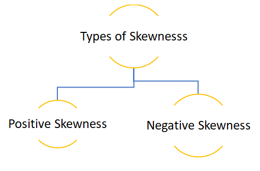
Skewness gives an idea about the shape of the distribution of your data. It helps you identify the side towards which your data is inclined. In such a case, the plot of the distribution is stretched to one side than to the other. This means in case of skewness we can say that the mean, median and mode of your dataset are not equal and does not follow the assumptions of a normally distributed curve.
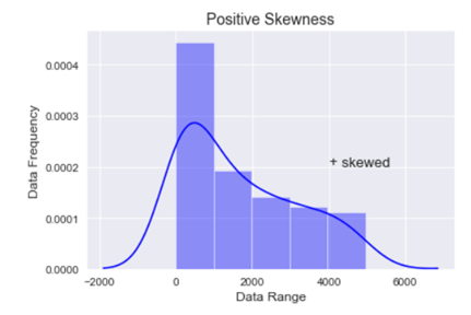
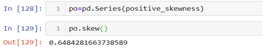
Positive skewness:- When the curve is stretched towards the right side more it is called a positively skewed curve. In this case mean is greater than median and median is the greater mode
(Mean>Median>Mode)
Let’s see how we can plot a positively skewed graph using python programming language.
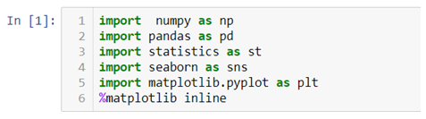
First we will have to import all the necessary libraries.
Then let’s create a data using the following code:-
In the above code we first created an empty list and then created a loop where we are generating a data of 100 observations. The initial value is raised by 0.1 and then each observation is raised by the loop count.
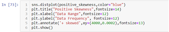
To get a visual representation of the above data we will be using the Seaborn library and to add more attributes to our graph we will use the Matplotlib methods.
In the above graph you can see that the data is stretched towards right, hence the data is positively skewed.
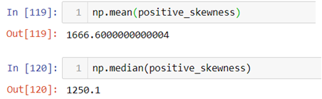
Now let’s cross validate the notion that whether Mean>Median>Mode or not.
Since each observation in the dataset is unique mode cannot be calculated.
Calculation of skewness:
Formula:-
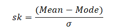
In case we have the value of mode then skewness can be measured by Mode ─ Mean
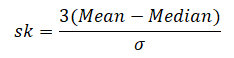
In case mode is ill-defined then skewness can be measured by 3(Mean ─ Median)
To obtain relative measures of skewness, as in dispersion we use the following formula:-
When mode is defined:- When mode is ill-defined:-
To calculate positive skewness using Python programming language we use the following code:-
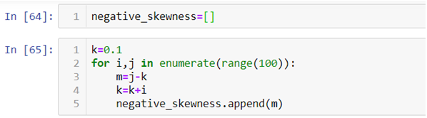
Negative skewness:- When the curve is stretched towards left side more it is called a negatively skewed curve. In this case mean is less than median and median is mode.
(Mean<Median<Mode)
Now let’s see how we can plot a negatively skewed graph using python programming language.
Since we have already imported all the necessary libraries we can head towards generating the data.|
In the above code instead of raising the value of observation we are reducing it.
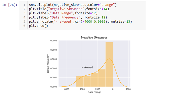
To visualize the data we have created again we will use the Seaborn and Matplotlib library.
The above graph is stretched towards left, hence it is negatively skewed.
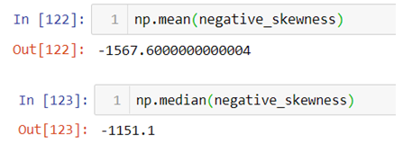
To check whether Mean<Median<Mode or not again we will be using the following code:-
The above result shows that the value of mean is less than mode and since each observation is unique mode cannot be calculated.
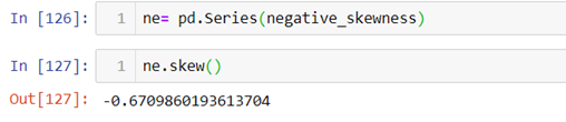
Now let’s calculate skewness in Python.
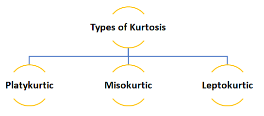
Kurtosis
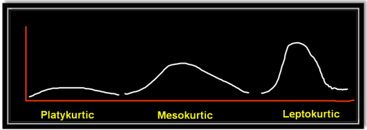
Kurtosis is nothing but the flatness or the peakness of a distribution curve.
Platykurtic :- This kind of distribution has the smallest or the flattest peak.
Misokurtic:- This kind of distribution has a medium peak.
Leptokurtic:- This kind of distribution has the highest peak.
The video attached below will help you clear any query you might have.
So, this was the discussion on the Skewness and Kurtosis, at the end of this you have definitely become familiar with both concepts. Dexlab Analytics blog has informative posts on diverse topics such as neural network machine learning python which you need to explore to update yourself. Dexlab Analytics offers cutting edge courses like machine learning certification courses in gurgaon.
In a world that is riveting towards exploring the hidden potential of emerging technologies like artificial intelligence, staying aware can not only keep you in sync but can also ensure your growth. Among all the tech terms doing the rounds now, machine learning is probably the one that you have heard frequently or, it might also be the term that intrigues you the most. You might even have a friend who is pursuing a Machine Learning course in Gurgaon. So, amidst all of this hoopla why don’t you upgrade your knowledge regarding machine learning? It’s not rocket science but, it’s science and it’s really cool!
Machine learning is a subset of AI that revolves round the concept of enabling a system to learn from the data automatically while finding patterns and improve the ability to predict without being explicitly programmed beforehand. One of the examples would be when you shop online from a particular site, you would notice product recommendations are lining up the page that particularly align with your preferences. The data footprint you leave behind is being picked up and analyzed to find a pattern and machine learning algorithms work to make predictions based on that, it is a continuous process of learning that simulate human learning process.
The same experience you would go through while watching YouTube, as it would present more videos based on your recent viewing pattern. Being such a powerful technology machine learning is gradually being implemented across different sectors and thereby pushing the demand for skilled personnel. Pursuing machine learning certification courses in gurgaon from a reputed institute, will enable an individual to pick up the nuances of machine learning to land the perfect career.
What are the different types of machine learning?
When we say machines learn, it might sound like a simple concept, but, the more you delve deeper into the topic to dissect the way it works you would know that there are more to it than meets the eyes. Machine learning could be divided into categories based on the learning aspect, here we will be focusing on 3 major categories which are namely:
Supervised Learning
Unsupervised Learning
Reinforcement Learning
Supervised Learning
Supervised learning as the name suggests involves providing the machine learning algorithm with training dataset, an example of sort to enable the system to learn to work its ways through to form the connection between input and output, the problem and the solution. The data provided for the training purposes needs to be correctly labeled so, that the algorithm is able to identify the relationship and could learn to predict output based on the input and upon finding errors could make necessary modifications. Post training when given a new dataset it should be able to analyze the input to predict a likely output for the new dataset. This basic form of machine learning is used for facial recognition, for classifying spams.
Unsupervised Learning
Again the term is suggestive like the prior category we discussed above, this is also the exact opposite of supervised learning as here there is no training data available to rely on. The input is available minus the output hence the algorithm does not have a reference to learn from. Basically the algorithm has to work its way through a big mass of unclassified data and start finding patterns on its own, due to the nature of its learning which involves parsing through unclassified data the process gets complicated yet holds potential. It basically involves clustering and association to work its way through data.
Reinforcement Learning
Reinforcement learning could be said to have similarity with the way humans learn through trial and error method. It does not have any guidance whatsoever and involves a reward, in a given situation the algorithm needs to work its way through to find the right solution to get to the reward, and it gets there by overcoming obstacles and learning from the errors along the way. The algorithm needs to analyze and find the best solution to maximize its rewards and minimize penalties as the process involves both. Video games could be an example of reinforcement learning.
Although only 3 core categories have been mentioned here, there remains other categories which deserve as much attention, such as deep learning. Deep learning too is a comparatively new field that deserves a complete discussion solely devoted to understanding this dynamic technology, focusing on its various aspects including how to be adept at deep learning for computer vision with python.
Machine learning is a highly potent technology that has the power to predict the future course of action, industries are waking up to smell the benefits that could be derived from implementation of ML. So, let’s quickly find out what some of the applications are:
Malware and spam filtering
You do not have to be tech savvy to understand what email spams are or, what malware is. Application of machine learning is refining the way emails are filtered with spams being detected and sent to a separate section, the same goes for malware detection as ML powered systems are quick to detect new malware from previous patterns.
Virtual personal assistants
As Alexa and Siri have become a part of life, we are now used to having access to our very own virtual personal assistants. However, when we ask a question or, give a command, ML starts working its magic as it gathers the data and processes it to offer a more personalized service by predicting the pattern of commands and queries.
Refined search results
When you put in a search query in Google or, any of the search engines the algorithms follow and learn from the pattern of the way you conduct a search and respond to the search results being displayed. Based on the patterns it refines the search results that impact page ranking.
Social media feeds
Whether it is Facebook or, Pinterest , the presence of machine learning could be felt across all platforms. Your friends, your interactions, your actions all of these are monitored and analyzed by machine learning algorithms to detect a pattern and prepare friend suggestions list. Automatic Friend Tagging Suggestions is another example of ML application.
Those were a couple of examples of machine learning application, but this dynamic field stretches far. The field is evolving and in the process creating new career opportunities. However, to land a job in this field one needs to have a background in Machine Learning Using Python, to become an expert and land the right job.
In this blog we will be introducing you to the Gaussian Distribution/Normal Distribution. Knowledge of the distribution of your data is quite important as it tells you the trend your data follows and a continuous observation of the trend helps you predict the future observations more accurately.
One of the most important distribution in statistics is Gaussian Distribution also known as Normal Distribution follows, that the mean, median and mode of the data are equal or almost equal. The idea behind this is that the data you collect should not have a very high standard deviation.
How to generate a normally distributed data in Python
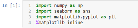
First we will import all the necessary libraries
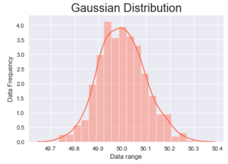
Now we will use .normal() method from Numpy library to generate the data where 50 is the mean, .1 is the deviation and 500 is the number of observations to be generated.
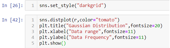
To plot the data and have a look at the data distribution we will be using .distplot() method from the Seaborn library and to make our plot visually better we will be using .set_style() method to change the background of our graph.
In the above line of codes we are also using Matplotlib library to add axis labels and title to the graph. We are also adding an argument fontsize to adjust the size of the font.
The above graph is a bell shaped curve with the peak of the curve in the center of the graph. This is one of the most important assumption of the Gaussian distribution on that the curve is symmetric at the center, some of the other assumptions are:-
Assumptions of the Gaussian distribution:
The mean, median and mode are equal.
Exactly half of the values are to the left of the center and exactly half of the values are to the right.
The total area under the curve is 1.
It has a continuous probability distribution.
68% of the data is -1 to 1 standard deviation away from the mean.
95% of the data is -2 to 2 standard deviation away from the mean.
99.7% of the data is -3 to 3 standard deviation away from the mean.
The last three assumptions can be proven with the help of standard normal distribution.
What is standard normal distribution?
Standard normal distribution also known as Z-score is a special case of normal distribution where we convert the normally distributed data into data deviations. The mean of such a distribution is 0 and the standard deviation is 1.
Let’s see how we can achieve the standard normal distribution in Python.
We will be using the same normally distributed data as above.
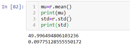
First we will be calculating the mean and standard deviation of the data we created with the help of the above code by using .mean() and .std() method.
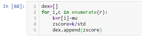
Now to calculate the Z-score we will first make an empty list and then append the calculated values one by one in that list with the help of a for-loop.
As you can see in the above code we are first subtracting the value from the mean and then dividing it by the standard deviation.
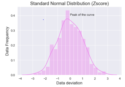
Now let’s see how the calculated data visually looks like.
When we look at the above graph we can clearly see that the data is by max 3 standard deviations away from the mean.
For further explanation check out the video attached down the blog.
So, with this we come to the end of today’s discussion on Gaussian distribution, hopefully, you found this explanation helpful. For such informative posts keep an eye on the Dexlab Analytics blog. Dexlab Analytics is a premier institute that offers cutting edge courses such as credit risk analysis course in Delhi.
Among all the decisions we make in our lives, choosing the right career path seems to be the most crucial one. Except for a couple of clueless souls, most students know by the time they clear their boards what they aspire to be. A big chunk of them veer towards engineering, MBA, even pursue masters degree in academics and post completion of their studies they settle for relevant jobs. So far that used to be the happily ever after career story, but, in the last couple of years there seems to be a big paradigm shift and it is causing a stir across industries. Professionals having an engineering background, or, masters degree are opting for a mid-career switch and a majority of them are opting for the data science domain by pursuing a Data Science course. So, what’s pushing them towards DS? Let’s investigate.
What’s causing the career switch?
No matter which field someone has chosen for career, achieving stability is a common goal. However, in many fields be it engineering, or, something else the job opportunities are not unlimited yet the number of job seekers is growing every year. So, thereby one can expect to face a stiff competition grabbing a well-paid job.
There have been many layoffs in recent times especially due to the unprecedented situation the world is going through. Even before that there were reports of job cuts and certain sectors not doing well would directly impact the career of thousands. Even if we do not concentrate on the extremes, the growth prospect in most places could be limited and achieving the desired salary or, promotion oftentimes becomes impossible. This leads to not only frustration but uncertainty as well.
The demand for big data
If you haven’t been living as a hermit, then you are aware of the data explosion that impacted nearly every industry. The moment everyone understood the power of big data they started investing in research and in building a system that can handle, store and process data which is a storehouse of information. Now, who is going to process data to extract the information? And here comes the new breed of data experts, namely the data scientists, who have mastered the technology having undergone Data Science training and are able to develop models and parse through data to deliver the insights companies are looking for to make informed decisions. The data trend is pushing the boundaries and as cutting edge technologies like AI, machine learning are percolating every aspect of the industries, the demand for avant-garde courses like natural language processing course in gurgaon, is skyrocketing.
Lack of trained industry ready data science professionals
Although big data has started trending as businesses started gathering data from multiple sources, there are not many professionals available to handle the data. The trend is only gaining momentum and if you just check the top job portals such as Glassdoor, Indeed and go through the ads seeking data scientists you would immediately know how far the field has traveled. With more and more industries turning to big data, the demand for qualified data scientists is shooting up.
Why data science is being chosen as the best option?
In the 21st century data science is a field which has plethora of opportunities for the right people and this is one field which is not only growing now but is also poised to grow in future as well. The data scientist is one of the most highest paid professional in today’s job market. According to the U.S. Bureau of Labor Statistics report by the year 2026 there is a possibility of creation of 11.5 million jobs in this field.
Now take a look at the Indian context, from agriculture to aviation the demand for data scientists would continue to grow as there is a severe shortage of professionals. As per a report the salary of a data scientist could hover around ₹1,052K per annum and remember the field is growing which means there is not going to be a dearth of job opportunities or, lucrative pay packages.
The shift
Considering all of these factors there has been a conscious shift in the mindset of the professionals, who are indeed making a beeline for institutes that offer data science certification. By doing so they hope to-
Access promising career opportunities
Achieve job satisfaction and financial stability
Earn more while enjoying job security
Work across industries and also be recruited by industry biggies
Gain valuable experience to be in demand for the rest of their career
Be a part of a domain that promises innovation and evolution instead of stagnation
Keeping in mind the growing demand for professionals and the dearth of trained personnel, premier institutes like DexLab Analytics have designed courses that are aimed to build industry-ready professionals. The best thing about such courses is that you can hail from any academic background, here you will be taught from scratch so that you can grasp the fundamentals before moving on to sophisticated modules.
Along with providing data science certification training, they also offer cutting edge courses such as, artificial intelligence certification in delhi ncr, Machine Learning training gurgaon. Such courses enable the professionals enhance their skillset to make their mark in a world which is being dominated by big data and AI. The faculty consists of skilled professionals who are armed with industry knowledge and hence are in a better position to shape students as per industry demands and standards.
The mid-career switch is happening and will continue to happen. There must be professionals who have the expertise to drive an organization towards the future by unlocking their data secrets. However, something must be kept in mind if you are considering a switch, you need to be ready to meet challenges, along with knowledge of Python for data science training, you need to have a vision, a hunger and a love for data to be a successful data scientist.
In this fifth part of the basic of statistical inference series you will learn about different types of Parametric tests. Parametric statistical test basically is concerned with making assumption regarding the population parameters and the distributions the data comes from. In this particular segment the discussion would focus on explaining different kinds of parametric tests. You can find the 4th part of the series here.
INTRODUCTION
Parametric statistics are the most common type of inferential statistics. Inferential statistics are calculated with the purpose of generalizing the findings of a sample to the population it represents, and they can be classified as either parametric or non-parametric. Parametric tests make assumptions about the parameters of a population, whereas nonparametric tests do not include such assumptions or include fewer. For instance, parametric tests assume that the sample has been randomly selected from the population it represents and that the distribution of data in the population has a known underlying distribution. The most common distribution assumption is that the distribution is normal. Other distributions include the binomial distribution (logistic regression) and the Poisson distribution (Poisson regression).
PARAMETRIC TEST
A parameter in statistics refers to an aspect of a population, as opposed to a statistic, which refers to an aspect, about a sample. For example, the population mean is a parameter, while the sample mean is a statistic. A parametric statistical test makes an assumption about the population parameters and the distributions that the data comes from. These types of tests assume to data is from normal distribution.
Data that is assumed to have been drawn from a particular distribution, and that is used in a parametric test.
Parametric equations are used in calculus to deal with the problems that arise when trying to find functions that describe curves. These equations are beyond the scope of this site, but you can find an excellent rundown of how to use these types of equations here.
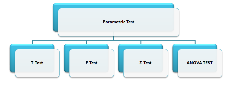
The parametric tests are: Let’s discuss about each test in details.
T-TEST
The T-test is one of, inferential statistics. It is used to determine whether there is a significant difference between the means of two groups or not. When the difference between two population averages is being investigated, a t-test is used. In other words, a t-test is used when we wish to compare two means. Essentially, a t-test allows us to compare the average values of the two data sets and determine if they came from the same population. In the above examples, if we were to take a sample of students from class A and another sample of students from class B, we would not expect them to have exactly the same mean and standard deviation.
Mathematically, the t-test takes a sample from each of the two sets and establishes the problem statement by assuming a null hypothesis that the two means are equal. Based on the applicable formulas, certain values are calculated and compared against the standard values, and the assumed null hypothesis is accepted or rejected accordingly.
If the null hypothesis qualifies to be rejected, it indicates that data readings are strong and are probably not due to chance. The t-test is just one of many tests used for this purpose. Statisticians must additionally use tests other than the t-test to examine more variables and tests with larger sample sizes. For a large sample size, statisticians use a z-test. Other testing options include the chi-square test and the f-test.
T-Test Assumptions
The first assumption made regarding t-tests concerns the scale of measurement. The assumption for a t-test is that the scale of measurement applied to the data collected follows a continuous or ordinal scale, such as the scores for an IQ test.
The second assumption made is that of a simple random sample, that the data is collected from a representative, randomly selected portion of the total population.
The third assumption is the data, when plotted, results in a normal distribution, bell-shaped distribution curve.
The final assumption is the homogeneity of variance. Homogeneous, or equal, variance exists when the standard deviations of samples are approximately equal.
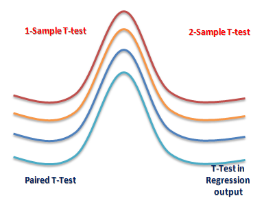
There are three types to T-test: (i) Correlated or paired T-test, (ii) Equal variance(or pooled) T-test (iii) Unequal variance T-test.
Z-TEST
A z-test is a statistical test used to determine whether two population means are different when the variances are known and the sample size is large. The test statistic is assumed to have a normal distribution, and nuisance parameters such as standard deviation should be known in order for an accurate z-test to be performed. A z-statistic, or z-score, is a number representing how many standard deviations above or below the mean population a score derived from a z-test is.
The z-test is also a hypothesis test in which the z-statistic follows a normal distribution. The z-test is best used for greater-than-30 samples because, under the central limit theorem, as the number of samples gets larger, the samples are considered to be approximately normally distributed. When conducting a z-test, the null and alternative hypotheses, alpha and z-score should be stated. Next, the test statistic should be calculated, and the results and conclusion stated. Examples of tests that can be conducted as z-tests include a one-sample location test, a two-sample location test, a paired difference test, and a maximum likelihood estimate. Z-tests are closely related to t-tests, but t-tests are best performed when an experiment has a small sample size. Also, t-tests assume the standard deviation is unknown, while z-tests assume it is known. If the standard deviation of the population is unknown, the assumption of the sample variance equaling the population variance is made.
One Sample Z-test: A one sample z test is one of the most basic types of hypothesis test. In order to run a one sample z test, its work through several steps:
Step 1: Null hypothesis is one of the common stumbling blocks–in order to make sense of your sample and have the one sample z test give you the right information it must make sure written the null hypothesis and alternate hypothesis correctly. For example, you might be asked to test the hypothesis that the mean weight gain of an women was more than 30 pounds. Your null hypothesis would be: H0 : μ = 30 and your alternate hypothesis would be H, sub>1: μ > 30.
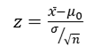
Step 2: Use the z-formula to find a z-score
All you do is put in the values you are given into the formula. Your question should give you the sample mean (x̄), the standard deviation (σ), and the number of items in the sample (n). Your hypothesized mean (in other words, the mean you are testing the hypothesis for, or your null hypothesis) is μ0 .
Two Sample Z Test: The z-Test: Two- Sample for Means tool runs a two sample z-Test means with known variances to test the null hypothesis that there is no difference between the means of two independent populations. This tool can be used to run a one-sided or two-sided test z-test.
ANOVA
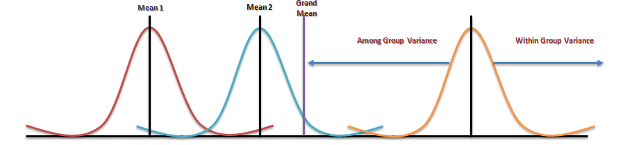
Analysis of variance (ANOVA) is an analysis tool used in statistics that splits an observed aggregate variability found inside a data set into two parts: systematic factors and random factors. The systematic factors have a statistical influence on the given data set, while the random factors do not. Analysts use the ANOVA test to determine the influence that independent variables have on the dependent variable in a regression study. The ANOVA test is the initial step in analysing factors that affect a given data set. Once the test is finished, an analyst performs additional testing on the methodical factors that measurably contribute to the data set’s inconsistency. The analyst utilizes the ANOVA test results in an f-test to generate additional data that aligns with the proposed regression models. The ANOVA test allows a comparison of more than two groups at the same time to determine whether a relationship exists between them. The result of the ANOVA formula, the F statistic (also called the F-ratio), allows for the analysis of multiple groups of data to determine the variability between samples and within samples.
If no real difference exists between the tested groups, which is called the null hypothesis, the result of the ANOVA’s F-ratio statistic will be close to 1. Fluctuations in its sampling will likely follow the Fisher F distribution. This is actually a group of distribution functions, with two characteristic numbers, called the numerator degrees of freedom and the denominator degrees of freedom.
One-way Anova: A one-way ANOVA uses one independent variable, use a one-way ANOVA when collected data about one categorical independent variable and one quantitative dependent variable. The independent variable should have at least three levels (i.e. at least three different groups or categories). ANOVA that if the dependent variable changes according to the level of the independent variable.
Two-way Anova: A two-way ANOVA is used to estimate how the mean of a quantitative variable changes according to the levels of two categorical variables. Use a two-way ANOVA when you want to know how two independent variables, in combination, affect a dependent variable.
F-TEST
An “F Test” is a catch-all term for any test that uses the F-distribution. In most cases, when people talk about the F-Test, what they are actually talking about is The F-Test to compare two variances. However, the f-statistic is used in a variety of tests including regression analysis, the Chow test and the Scheffe Test (a post-hoc ANOVA test).
F Test to Compare Two Variances
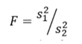
A Statistical F Test uses an F Statistic to compare two variances, s1 and s2 , by dividing them. The result is always a positive number (because variances are always positive). The equation for comparing two variances with the f-test is:
If the variances are equal, the ratio of the variances will equal 1. For example, if you had two data sets with a sample 1 (variance of 10) and a sample 2 (variance of 10), the ratio would be 10/10 = 1.
You always test that the population variances are equal when running an F Test. In other words, you always assume that the variances are equal to 1. Therefore, your null hypothesis will always be that the variances are equal. Assumptions
Several assumptions are made for the test. Your population must be approximately normally distributed (i.e. fit the shape of a bell curve) in order to use the test. Plus, the samples must be independent events. In addition, you’ll want to bear in mind a few important points:
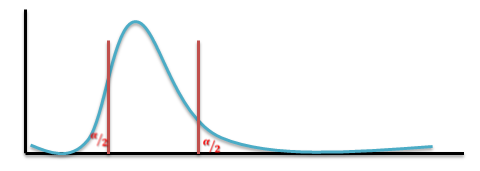
The larger variance should always go in the numerator (the top number) to force the test into a right-tailed test. Right-tailed tests are easier to calculate.
For two-tailed tests, divide alpha by 2 before finding the right critical value.
If you are given standard deviations, they must be squared to get the variances.
If your degrees of freedom aren’t listed in the F Table, use the larger critical value. This helps to avoid the possibility of Type I errors.
CONCLUSION
Conventional statistical procedures may also call parametric tests. In every parametric test, for example, you have to use statistics to estimate the parameter of the population. Because of such estimation, you have to follow a process that includes a sample as well as a sampling distribution and a population along with certain parametric assumptions that required, which makes sure that all components compatible with one another.
An example can use to explain this. Observations are first of all quite independent, the sample data doesn’t have any normal distributions and the scores in the different groups have some homogeneous variances. Parametric tests are based on the distribution, parametric statistical tests are only applicable to the variables. There’re no parametric tests that exist for the nominal scale date, and finally, they are quite powerful when they exist. There are mainly four types of Parametric Hypothesis Test which already mentioned in previous slides.
Advantages of Parametric Test
One of the biggest and best advantages of using parametric tests is first of all that you don’t need much data that could be converted in some order or format of ranks. The process of conversion is something that appears in rank format and to be able to use a parametric test regularly, you will end up with a severe loss in precision. Another big advantage of using parametric tests is the fact that you can calculate everything so easily. In short, you will be able to find software much quicker so that you can calculate them fast and quick. Apart from parametric tests, there are other non-parametric tests, where the distributors are quite different and they are not all that easy when it comes to testing such questions that focus related to the means and shapes of such distributions.
Disadvantages of Parametric Test
Parametric tests are not valid when it comes to small data sets. The requirement that the populations are not still valid on the small sets of data, the requirement that the populations which are under study have the same kind of variance and the need for such variables are being tested and have been measured at the same scale of intervals. Another disadvantage of parametric tests is that the size of the sample is always very big, something you will not find among non-parametric tests. That makes it a little difficult to carry out the whole test.
This particular discussion on parametric tests ends here, and at the end of this you must have developed clear ideas regarding these test categories. To find more such posts on Data Science training topics follow the Dexlab Analytics blog.
In this series we cover the basic of statistical inference, this is the fourth part of our discussion where we explain the concept of hypothesis testing which is a statistical technique. You could also check out the 3rd part of the series here.
Introduction
The objective of sampling is to study the features of the population on the basis of sample observations. A carefully selected sample is expected to reveal these features, and hence we shall infer about the population from a statistical analysis of the sample. This process is known as Statistical Inference.
There are two types of problems. Firstly, we may have no information at all about some characteristics of the population, especially the values of the parameters involved in the distribution, and it is required to obtain estimates of these parameters. This is the problem of Estimation. Secondly, some information or hypothetical values of the parameters may be available, and it is required to test how far the hypothesis is tenable in the light of the information provided by the sample. This is the problem of Test of Hypothesis or Test of Significance.
In many practical problems, statisticians are called upon to make decisions about a population on the basis of sample observations. For example, given a random sample, it may be required to decide whether the population, from which the sample has been obtained, is a normal distribution with mean = 40 and s.d. = 3 or not. In attempting to reach such decisions, it is necessary to make certain assumptions or guesses about the characteristics of population, particularly about the probability distribution or the values of its parameters. Such an assumption or statement about the population is called Statistical Hypothesis. The validity of a hypothesis will be tested by analyzing the sample. The procedure which enables us to decide whether a certain hypothesis is true or not, is called Test of Significance or Test of Hypothesis.
What Is Testing Of Hypothesis?
Statistical Hypothesis
Hypothesis is a statistical statement or a conjecture about the value of a parameter. The basic hypothesis being tested is called the null hypothesis. It is sometimes regarded as representing the current state of knowledge & belief about the value being tested. In a test the null hypothesis is constructed with alternative hypothesis denoted by 𝐻1 ,when a hypothesis is completely specified then it is called a simple hypothesis, when all factors of a distribution are not known then the hypothesis is known as a composite hypothesis.
Testing Of Hypothesis
The entire process of statistical inference is mainly inductive in nature, i.e., it is based on deciding the characteristics of the population on the basis of sample study. Such a decision always involves an element of risk i.e., the risk of taking wrong decisions. It is here that modern theory of probability plays a vital role & the statistical technique that helps us at arriving at the criterion for such decision is known as the testing of hypothesis.
Testing Of Statistical Hypothesis
A test of a statistical hypothesis is a two action decision after observing a random sample from the given population. The two action being the acceptance or rejection of hypothesis under consideration. Therefore a test is a rule which divides the entire sample space into two subsets.
A region is which the data is consistent with 𝐻0.
The second is its complement in which the data is inconsistent with 𝐻0.
The actual decision is however based on the values of the suitable functions of the data, the test statistic. The set of all possible values of a test statistic which is consistent with 𝐻0 is the acceptance region and all these values of the test statistic which is inconsistent with 𝐻0 is called the critical region. One important condition that must be kept in mind for efficient working of a test statistic is that the distribution must be specified.
Does the acceptance of a statistical hypothesis necessarily imply that it is true?
The truth a fallacy of a statistical hypothesis is based on the information contained in the sample. The rejection or the acceptance of the hypothesis is contingent on the consistency or inconsistency of the 𝐻0 with the sample observations. Therefore it should be clearly bowed in mind that the acceptance of a statistical hypothesis is due to the insufficient evidence provided by the sample to reject it & it doesn’t necessarily imply that it is true.
Elements: Null Hypothesis, Alternative Hypothesis, Pot
Null Hypothesis
A Null hypothesis is a hypothesis that says there is no statistical significance between the two variables in the hypothesis. There is no difference between certain characteristics of a population. It is denoted by the symbol 𝐻0. For example, the null hypothesis may be that the population mean is 40 then
𝐻0(𝜇 = 40)
Let us suppose that two different concerns manufacture drugs for including sleep, drug A manufactured by first concern and drug B manufactured by second concern. Each company claims that its drug is superior to that of the other and it is desired to test which is a superior drug A or B? To formulate the statistical hypothesis let X be a random variable which denotes the additional hours of sleep gained by an individual when drug A is given and let the random variable Y denote the additional hours to sleep gained when drug B is used. Let us suppose that X and Y follow the probability distributions with means 𝜇𝑥 and 𝜇𝑌 respectively.
Here our null hypothesis would be that there is no difference between the effects of two drugs. Symbolically,
𝐻0: 𝜇𝑋 = 𝜇𝑌
Alternative Hypothesis
A statistical hypothesis which differs from the null hypothesis is called an Alternative Hypothesis, and is denoted by 𝐻1. The alternative hypothesis is not tested, but its acceptance (rejection) depends on the rejection (acceptance) of the null hypothesis. Alternative hypothesis contradicts the null hypothesis. The choice of an appropriate critical region depends on the type of alternative hypothesis, whether both-sided, one-sided (right/left) or specified alternative.
Alternative hypothesis is usually denoted by 𝐻1.
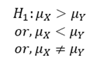
For example, in the drugs problem, the alternative hypothesis could be
Power Of Test
The null hypothesis 𝐻0 𝜃 = 𝜃0 is accepted when the observed value of test statistic lies the critical region, as determined by the test procedure. Suppose that the true value of 𝜃 is not 𝜃0, but another value 𝜃1, i.e. a specified alternative hypothesis 𝐻1 𝜃 = 𝜃1 is true. Type II error is committed if 𝐻0 is not rejected, i.e. the test statistic lies outside the critical region. Hence the probability of Type II error is a function of 𝜃1, because now 𝜃 = 𝜃1 is assumed to be true. If 𝛽 𝜃1 denotes the probability of Type II error, when 𝜃 = 𝜃1 is true, the complementary probability 1 − 𝛽 𝜃1 is called power of the test against the specified alternative 𝐻1 𝜃 = 𝜃1 . Power = 1-Probability of Type II error=Probability of rejection 𝐻0 when 𝐻1 is true Obviously, we could like a test to be as ‘powerful’ as possible for all critical regions of the same size. Treated as a function of 𝜃, the expression of 𝑃 𝜃 = 1 − 𝛽 𝜃 is called Power Function of the test for 𝜃0 against 𝜃. the curve obtained by plotting P(𝜃) against all possible values of 𝜃, is known as Power Curve.
Elements: Type I & Type II Error
Type I Error & Type Ii Error
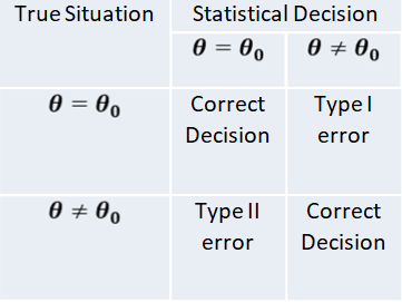
The procedure of testing statistical hypothesis does not guarantee that all decisions are perfectly accurate. At times, the test may lead to erroneous conclusions. This is so, because the decision is taken on the basis of sample values, which are themselves fluctuating and depend purely on chance. The errors in statistical decisions are two types:
Type I Error – This is the error committed by the test in rejecting a true null hypothesis.
Type II Error – This is the error committed by the test in accepting a false null hypothesis.
Considering for the population mean is 40, i.e. 𝐻0 𝜇 = 40 , let us imagine that we have a random sample from a population whose mean is really 40. if we apply the test for 𝐻0 𝜇 = 40 , we might find that the values of test statistic lines in the critical region, thereby leading to the conclusion that the population mean is not 40; i.e. the test rejects the null hypothesis although it is true. We have thus committed what is known as “Type I error” or “Error of first kind”. On the other hand, suppose that we have a random sample from a population whose mean is known to different from 40, say 43. if we apply the test for 𝐻0 𝜇 = 40 , the value of the statistic may, by chance, lie in the acceptance region, leading to the conclusion that the mean may be 40; i.e. the test does not reject the null hypothesis 𝐻0 𝜇 = 40 , although it is false. This is again another form of incorrect decision, and the error thus committed is known as “Type II error” or “Error of second kind”.
Using sampling distribution of the test statistic, we can measure in advance the probabilities of committing the two types of error. Since the null hypothesis is rejected only when the test statistic falls in the critical region.
Probability of Type I error = Probability of rejecting 𝐻0 𝜃 = 𝜃0 , when it is true = Probability that the test statistic lies in the critical region, assuming 𝜃 = 𝜃0.
The probability of Type I error must not exceed the level of significance (𝛼) of the test.
The probability of Type II error assumes different values for different values of 𝜃 covered by the alternative hypothesis 𝐻1. Since the null hypothesis is accepted only when the observed value of the best statistic lies outside the critical region.
Probability of Type II error 𝑊ℎ𝑒𝑛 𝜃 = 𝜃1 = Probability of accepting 𝐻0 𝜃 = 𝜃0 , when it is false = Probability that the test statistic lies in the region of acceptance, assuming 𝜃 = 𝜃1
The probability of Type I error is necessary for constructing a test of significance. It is in fact the ‘size of the Critical Region’. The probability of Type II error is used to measure the “power” of the test in detecting falsity of the null hypothesis. When the population has a continuous distribution
Probability of Type I error = Level of significance = Size of critical region
Elements: Level Of Significance & Critical Region
Level Of Significance And Critical Region
The decision about rejection or otherwise of the null hypothesis is based on probability considerations. Assuming the null hypothesis to be true, we calculate the probability of obtaining a difference equal to or greater than the observed difference. If this probability is found to be small, say less than .05, the conclusion is that the observed value of the statistic is rather unusual and has been caused due to the underlying assumption (i.e. null hypothesis) that is not true. We say that the observed difference is significant at 5 per cent level, and hence the ‘null hypothesis is rejected’ at 5 per cent level of significance. If, however, this probability is not very small, say more than .05, the observed difference cannot be considered to be unusual and is attributed to sampling fluctuation only. The difference is, now said to be not significant at 5 per cent level, and we conclude that there is no reason to reject the null hypothesis’ at 5 per cent level of significance. It has become customary to use 5% and 1% level of significance, although other levels, such as 2% or 5% may also be used.
Without actually going to calculate this probability, the test of significance may be simplified as follows. From the sampling distribution of the statistic, we find the maximum difference is which is exceeded in (say 5) percent of cases. If the observed difference in larger than this value, the null hypothesis is rejected. It is less there in no reason to reject the null hypothesis.
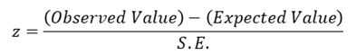
Suppose, the sampling distribution of the statistic is a normal distribution. Since the area under normal curve outside the ordinates at mean ±1.96 (𝑠. 𝑑. ) is only 5%, the probability that the observed value of the statistic differs from the expected value of 1.96 times the S.E. or more is .05; and the probability of a larger difference will be still smaller. If, therefore
Is either greater than 1.96 or less than -1.96 (i.e. numerically greater than 1.96), the null hypothesis 𝐻0 is rejected at 5% level of significance. The set values 𝑧 ≥ 1.96 𝑜𝑟 ≤ −1.96, i.e.
|𝑧| ≥ 1.96
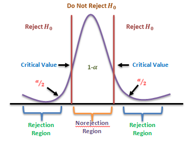
constitutes what is called the Critical Region for the test. Similarly since the area outside mean ±2.58 (s.d.) is only 1%. 𝐻0 is rejected at 1% level of significance, if z numerically exceeds 258, i.e. the critical region is 𝑧 ≥ 2.58 at 1% level. Using the sampling distribution of an appropriate test statistic we are able to establish the maximum difference at a specified level between the observed and expected values that is consistent with null hypothesis 𝐻0 . The set of values of the test statistic corresponding to this difference which lead to the acceptance of 𝐻0 is called Region of acceptance. Conversely, the set of values of the statistic leading to the rejection of 𝐻0 is referred to as Region of Rejection or “Critical Region” of the test. The value of the statistic which lies at the boundary of the regions of acceptance and the rejection is called Critical value. When the null hypothesis is true, the probability of observed value of the test statistic falling in the critical region is often called the “Size of Critical Region”.
𝑆𝑖𝑧𝑒 𝑜𝑓 𝐶𝑟𝑖𝑡𝑖𝑐𝑎𝑙 𝑅𝑒𝑔𝑖𝑜𝑛 ≤ 𝐿𝑒𝑣𝑒𝑙 𝑜𝑓 𝑆𝑖𝑔𝑛𝑖𝑓𝑖𝑐𝑎𝑛𝑐𝑒
However, for a continuous population, the critical region is so determined that its size equals the Level of Significance (𝛼).
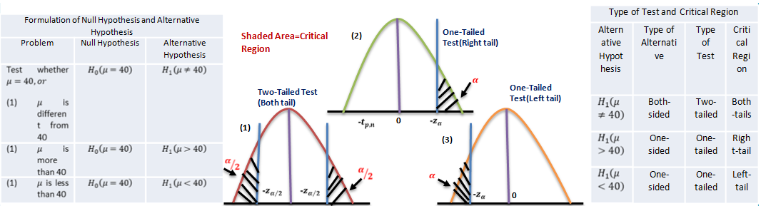
Two-Tailed And One-Tailed Tests
Our discussion above were centered around testing the significance of ‘difference’ between the observed and expected values, i.e. whether the observed value is significantly different from (i.e. either larger or smaller than) the expected value, as could arise due to fluctuations of random sampling. In the illustration, the null hypothesis is tested against “both-sided alternatives” 𝜇 > 40 𝑜𝑟 𝜇 < 40 , i.e.
𝐻0 𝜇 = 40 𝑎𝑔𝑎𝑖𝑛𝑠𝑡 𝐻1 𝜇 ≠ 40
Thus assuming 𝐻0 to be true, we would be looking for large differences on both sides of the expected value, i.e. in “both tails” of the distribution. Such tests are, therefore, called “Two-tailed tests”.
Sometimes we are interested in tests for large differences on one side only i.e., in one ‘one tail’ of the distribution. For example, whether a change in the production bricks with a ‘higher’ breaking strength, or whether a change in the production technique yields ‘lower’ percentage of defectives. These are known as “One-tailed tests”.
For testing the null hypothesis against “one-sided alternatives (right side)” 𝜇 > 40 , i.e.
𝐻0 𝜇 = 40 𝑎𝑔𝑎𝑖𝑛𝑠𝑡𝐻1 𝜇 > 40
The calculated value of the statistic z is compared with 1.645, since 5% of the area under the standard normal curve lies to the right of 1.645. if the observed value of z exceeds 1.645, the null hypothesis 𝐻0 is rejected at 5% level of significance. If a 1% level were used, we would replace 1.645 by 2.33. thus the critical regions for test at 5% and 1% levels are 𝑧 ≥ 1.645 and 𝑧 ≥ 2.33 respectively.
For testing the null hypothesis against “one-sided alternatives (left side)” 𝜇 < 40 i.e.
𝐻0 𝜇 = 40 𝑎𝑔𝑎𝑖𝑛𝑠𝑡𝐻1 𝜇 < 40
The value of z is compared with -1.645 for significance at 5% level, and with -2.33 for significance at 1% level. The critical regions are now 𝑧 ≤ −1.645 and 𝑧 ≤ −2.33 for 5% and 1% levels respectively. In fact, the sampling distributions of many of the commonly-used statistics can be approximated by normal distributions as the sample size increases, so that these rules are applicable in most cases when the sample size is ‘large’, say, more than 30. It is evident that the same null hypothesis may be tested against alternative hypothesis of different types depending on the nature of the problem. Correspondingly, the type of test and the critical region associated with each test will also be different.
Solving Testing Of Hypothesis Problem
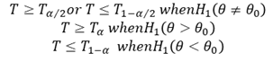
Step 1 Set up the “Null Hypothesis” 𝐻0 and the “Alternative Hypothesis” 𝐻1 on the basis of the given problem. The null hypothesis usually specifies the values of some parameters involved in the population: 𝐻0 𝜃 = 𝜃0 . The alternative hypothesis may be any one of the following types: 𝐻1 ( ) 𝜃 ≠ 𝜃1 𝐻1 𝜃 > 𝜃0 , 𝐻1 𝜃 < 𝜃0 . The types of alternative hypothesis determines whether to use a two-tailed or one-tailed test (right or left tail).
Step 2
State the appropriate “test statistic” T and also its sampling distribution, when the null hypothesis is true. In large sample tests the statistic 𝑧 = (𝑇 − 𝜃0)Τ𝑆. 𝐸. , (T) which approximately follows Standard Normal Distribution, is often used. In small sample tests, the population is assumed to be Normal and various test statistics are used which follow Standard Normal, Chi-square, t for F distribution exactly.
Step 3 Select the “level of significance” 𝛼 of the test, if it is not specified in the given problem. This represents the maximum probability of committing a Type I error, i.e., of making a wrong decision by the test procedure when in fact the null hypothesis is true. Usually, a 5% or 1% level of significance is used (If nothing is mentioned, use 5% level).
Step 4
Find the “Critical region” of the test at the chosen level of significance. This represents the set of values of the test statistic which lead to rejection of the null hypothesis. The critical region always appears in one or both tails of the distribution, depending on weather the alternative hypothesis is one-sided or both-sided. The area in the tails must be equal to the level of significance 𝛼. For a one-tailed test, 𝛼 appears in one tail and for two-tailed test 𝛼/2 appears in each tail of the distribution. The critical region is
Where 𝑇𝛼 is the value of T such that the area to its tight is 𝛼.
Step 5
Compute the value of the test statistic T on the basis of sample data the null hypothesis. In large sample tests, if some parameters remain unknown they should be estimated from the sample. Step 6
If the computed value of test statistic T lies in the critical region, “reject 𝐻0”; otherwise “do not reject 𝐻0 ”. The decision regarding rejection or otherwise of 𝐻0 is made after a comparison of the computed value of T with critical value (i.e., boundary value of the appropriate critical region).
Step 7 Write the conclusion in plain non-technical language. If 𝐻0 is rejected, the interpretation is: “the data are not consistent with the assumption that the null hypothesis is true and hence 𝐻0 is not tenable”. If 𝐻0 is not rejected, “the data cannot provide any evidence against the null hypothesis and hence 𝐻0 may be accepted to the true”. The conclusion should preferably be given in the words stated in the problem.
Conclusion
Hypothesis is a statistical statement or a conjecture about the value of a parameter. The legal concept that one is innocent until proven guilty has an analogous use in the world of statistics. In devising a test, statisticians do not attempt to prove that a particular statement or hypothesis is true. Instead, they assume that the hypothesis is incorrect (like not guilty), and then work to find statistical evidence that would allow them to overturn that assumption. In statistics this process is referred to as hypothesis testing, and it is often used to test the relationship between two variables. A hypothesis makes a prediction about some relationship of interest. Then, based on actual data and a pre-selected level of statistical significance, that hypothesis is either accepted or rejected. There are some elements of hypothesis like null hypothesis, alternative hypothesis, type I & type II error, level of significance, critical region and power of test and some processes like one and two tail test to find the critical region of the graph as well as the error that help us reach the final conclusion.
A Null hypothesis is a hypothesis that says there is no statistical significance between the two variables in the hypothesis. There is no difference between certain characteristics of a population. It is denoted by the symbol 𝐻0. A statistical hypothesis which differs from the null hypothesis is called an Alternative Hypothesis, and is denoted by 𝐻1. The procedure of testing statistical hypothesis does not guarantee that all decisions are perfectly accurate. At times, the test may lead to erroneous conclusions. This is so, because the decision is taken on the basis of sample values, which are themselves fluctuating and depend purely on chance, this process called types of error. Hypothesis testing is very important part of statistical analysis. By the help of hypothesis testing many business problem can be solved accurately.
That was the fourth part of the series, that explained hypothesis testing and hopefully it clarified your notion of the same by discussing each crucial aspect of it. You can find more informative posts like this one on Data Science course topics. Just keep on following the Dexlab Analytics blog to stay informed.
When we take a look at a video or, a bunch of images we know what’s what just by taking one look, it is our innate ability that gradually developed. Well, sophisticated technologies such as object detection can do that too. It might sound futuristic but it is happening now in reality. Object detection is a technique of the AI subset computer vision that is concerned with identifying objects and defining those by placing into distinct categories such as humans, cars, animals etc.
It combines machine learning and deep learning to enable machines to identify different objects. However, image recognition and object detection these terms are often used interchangeably but, both techniques are different. Object detection could detect multiple objects in an image or, in a video. The demand for trained experts in this field is pretty high and having a background in deep learning for computer vision with python can help one build a dream career.
Object detection has found applications across industries. Let’s take a look at some of these applications.
Tracking objects
It is needless to point out that in the field of security and surveillance object detection would play an even more important role. With object tracking it would be easier to track a person in a video. Object tracking could also be used in tracking the motion of a ball during a match. In the field of traffic monitoring too object tracking plays a crucial role.
Counting the crowd
Crowd counting or people counting is another significant application of object detection. During a big festival, or, in a crowded mall this application comes in handy as it helps in dissecting the crowd and measure different groups.
Self-driving cars
Another unique application of object detection technique is definitely self-driving cars. A self-driving car can only navigate through a street safely if it could detect all the objects such as people, other cars, road signs on the road, in order to decide what action to take.
Detecting a vehicle
In a road full of speeding vehicles object detection can help in a big way by tracking a particular vehicle and even its number plate. So, if a car gets into an accident or, breaks traffic rules then it is easier to detect that particular car using object detection model and thereby decreasing the rate of crime while enhancing security.
Detecting anomaly
Another useful application of object detection is definitely spotting an anomaly and it has industry specific usages. For instance, in the field of agriculture object detection helps in identifying infected crops and thereby helps the farmers take measures accordingly. It could also help identify skin problems in healthcare. In the manufacturing industry the object detection technique can help in detecting problematic parts really fast and thereby allow the company to take the right step.
Object detection technology has the potential to transform our world in multiple ways. However, the models still need to be developed further so that these can be applied across devices and platforms in real-time to offer cutting-edge solutions. Pursuing a Python Certification course can help develop the required skills needed for making a career in the field of machine learning.