
In this blog we will be introducing you to the Gaussian Distribution/Normal Distribution. Knowledge of the distribution of your data is quite important as it tells you the trend your data follows and a continuous observation of the trend helps you predict the future observations more accurately.
One of the most important distribution in statistics is Gaussian Distribution also known as Normal Distribution follows, that the mean, median and mode of the data are equal or almost equal. The idea behind this is that the data you collect should not have a very high standard deviation.
How to generate a normally distributed data in Python
- First we will import all the necessary libraries
- Now we will use .normal() method from Numpy library to generate the data where 50 is the mean, .1 is the deviation and 500 is the number of observations to be generated.
![]()
- To plot the data and have a look at the data distribution we will be using .distplot() method from the Seaborn library and to make our plot visually better we will be using .set_style() method to change the background of our graph.
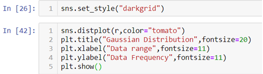
In the above line of codes we are also using Matplotlib library to add axis labels and title to the graph. We are also adding an argument fontsize to adjust the size of the font.
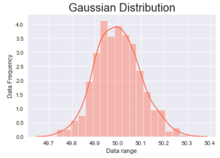
The above graph is a bell shaped curve with the peak of the curve in the center of the graph. This is one of the most important assumption of the Gaussian distribution on that the curve is symmetric at the center, some of the other assumptions are:-
Assumptions of the Gaussian distribution:
- The mean, median and mode are equal.
- Exactly half of the values are to the left of the center and exactly half of the values are to the right.
- The total area under the curve is 1.
- It has a continuous probability distribution.
- 68% of the data is -1 to 1 standard deviation away from the mean.
- 95% of the data is -2 to 2 standard deviation away from the mean.
- 99.7% of the data is -3 to 3 standard deviation away from the mean.
The last three assumptions can be proven with the help of standard normal distribution.
What is standard normal distribution?
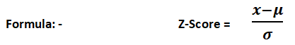
Standard normal distribution also known as Z-score is a special case of normal distribution where we convert the normally distributed data into data deviations. The mean of such a distribution is 0 and the standard deviation is 1.
Let’s see how we can achieve the standard normal distribution in Python.
We will be using the same normally distributed data as above.
![]()
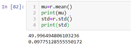
- First we will be calculating the mean and standard deviation of the data we created with the help of the above code by using .mean() and .std() method.
- Now to calculate the Z-score we will first make an empty list and then append the calculated values one by one in that list with the help of a for-loop.
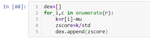
As you can see in the above code we are first subtracting the value from the mean and then dividing it by the standard deviation.
Now let’s see how the calculated data visually looks like.
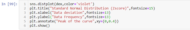
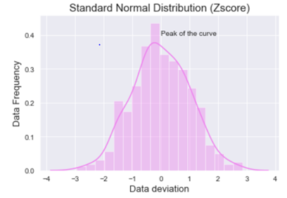
When we look at the above graph we can clearly see that the data is by max 3 standard deviations away from the mean.
For further explanation check out the video attached down the blog.
So, with this we come to the end of today’s discussion on Gaussian distribution, hopefully, you found this explanation helpful. For such informative posts keep an eye on the Dexlab Analytics blog. Dexlab Analytics is a premier institute that offers cutting edge courses such as credit risk analysis course in Delhi.
Niharika Rai
Analytics Consultant, DexLab Analytics
.
Python, Python certification, python certification course, Python courses